11 Essential Ways to Determine Normality of Data Distributions
A guide to plotting, statistical and distance methods.
Many ML models assume (or work better) under the presence of normal distribution.
For instance:
Linear regression assumes residuals are normally distributed.
At times, transforming the data to normal distribution can be beneficial.
Linear discriminant analysis (LDA) is derived under the assumption of normal distribution, etc.
Thus, being aware of the ways to test normality is extremely crucial for data scientists.
The visual below depicts the 11 essential ways to test normality.
Let’s understand these today.
#1) Plotting Methods (self-explanatory)
Histogram
QQ Plot (We covered it yesterday here: QQ Plot)
KDE Plot
Violin Plot
While plotting is often reliable, it is a subjective approach and prone to errors.
Thus, we must know reliable quantitative measures as well.
#2) Statistical Methods:
Shapiro-Wilk test:
Finds a statistic using the correlation between the observed data and the expected values under a normal distribution.
The p-value indicates the likelihood of observing such a correlation if the data were normally distributed.
A high p-value indicates a normal distribution.
Get started: Scipy Docs.
KS test:
Measures the max difference between the cumulative distribution functions (CDF) of observed and normal distribution.
The output statistic is based on the max difference between the two CDFs.
A high p-value indicates a normal distribution.
Get started: Scipy Docs.
Anderson-Darling test:
Measures the differences between the observed data and the expected values under a normal distribution.
Emphasizes the differences in the tail of the distribution.
This makes it particularly effective at detecting deviations in the extreme values.
Get started: Scipy Docs.
Lilliefors test:
It is a modification of the KS test.
The KS test is appropriate in situations where the parameters of the reference distribution are known.
If the parameters are unknown, Lilliefors is recommended.
Get started: Statsmodel Docs.
#3) Distance Measures
Distance measures are another reliable and more intuitive way to test normality.
But they can be a bit tricky to use.
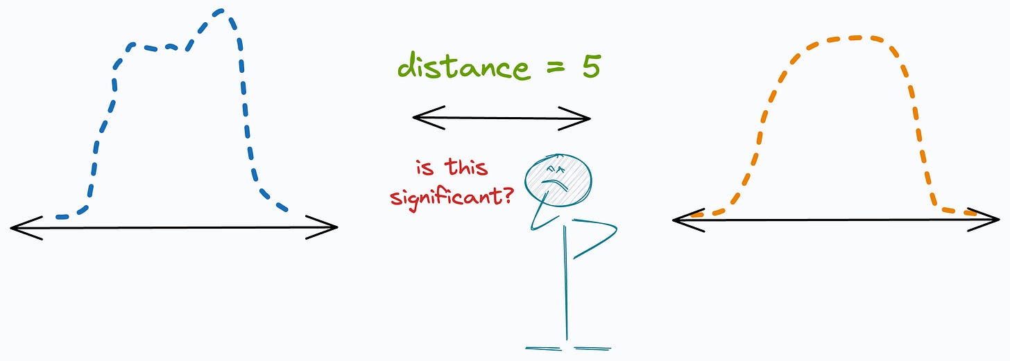
See, the problem is that a single distance value needs more context for interpretability.
For instance, if the distance between two distributions is 5, is this large or small?
We need more context.
I prefer using these measures as follows:
Find the distance between the observed distribution and multiple reference distributions.
Select the reference distribution with the minimum distance to the observed distribution.
Here are a few distance common and useful measures:
Bhattacharyya distance:
Measure the overlap between two distributions.
This “overlap” is often interpreted as closeness between two distributions.
Choose the distribution that has the least Bhattacharyya distance to the observed distribution.
We covered it in detail here: Bhattacharyya Distance.
Hellinger distance (Shout out to Joe Corliss for introducing this to me):
It is used quite similar to how we use the Bhattacharyya distance
The difference is that Bhattacharyya distance does not satisfy triangular inequality.
But Hellinger distance does.
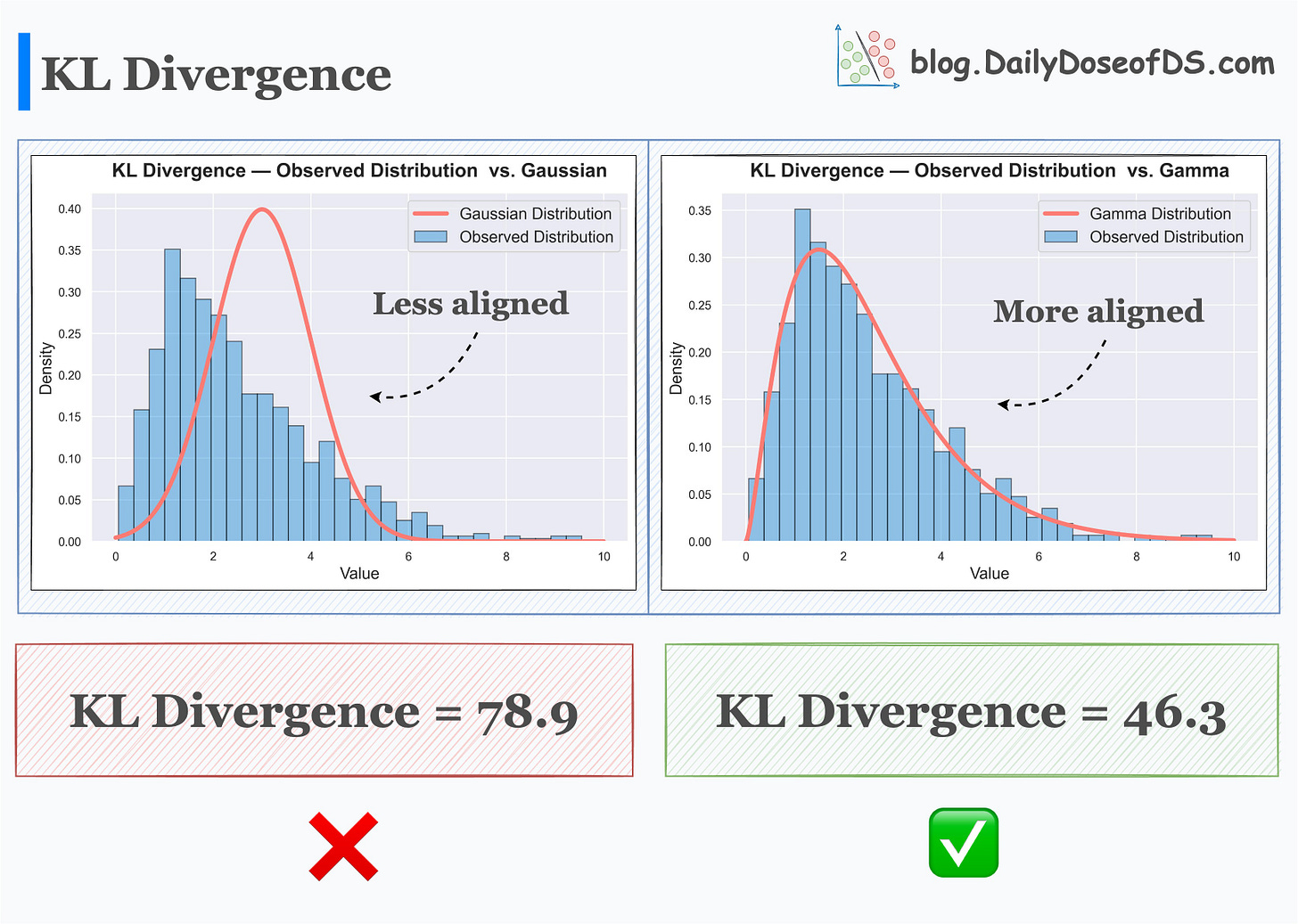
KL Divergence:
It is not entirely a "distance metric" per se, but can be used in this case.
Measure information lost when one distribution is approximated using another distribution.
The more information is lost, the more the KL Divergence.
Choose the distribution that has the least KL divergence from the observed distribution.
We covered it in detail here: KL Divergence.
👉 Over to you: What other common methods have I missed?
👉 If you liked this post, don’t forget to leave a like ❤️. It helps more people discover this newsletter on Substack and tells me that you appreciate reading these daily insights.
The button is located towards the bottom of this email.
Thanks for reading!
Latest full articles
If you’re not a full subscriber, here’s what you missed last month:
You Cannot Build Large Data Projects Until You Learn Data Version Control!
Why Bagging is So Ridiculously Effective At Variance Reduction?
Sklearn Models are Not Deployment Friendly! Supercharge Them With Tensor Computations.
Deploy, Version Control, and Manage ML Models Right From Your Jupyter Notebook with Modelbit
Model Compression: A Critical Step Towards Efficient Machine Learning.
Gaussian Mixture Models (GMMs): The Flexible Twin of KMeans.
To receive all full articles and support the Daily Dose of Data Science, consider subscribing:
👉 Tell the world what makes this newsletter special for you by leaving a review here :)
👉 If you love reading this newsletter, feel free to share it with friends!


Great article! I remember that Shapiro-Wilk had some kind of limitation about if n < 50, if I am not wrong.
This is great info, but I would also like to see the limitations of each method and a tip of when is best to use which. Unfortunately there are so many ways to do it, the experience of WHEN to use which or the PREFERENCE to use a preferred method are what I am most interested in. For example of all the methods shown, which works the most often, then when x happens what is the second best to diverge too... like a decision tree for implementation would be awesome!