11 Key Probability Distributions in Data Science

Essential for statistical modeling.

Apr 20, 2024

Advertise | Deep Dives | Student Discount

Statistical models assume an underlying data generation process.

This is exactly what lets us formulate the generation process, using which we define the maximum likelihood estimation (MLE) step.

What is MLE?

Feel free to skip this part if you already know what is MLE.

Simply put, MLE is a method for estimating the parameters of a statistical model by maximizing the likelihood of the observed data.

More formally, a model attempts to find the specific set of parameters (θ), which maximizes the likelihood function (L):

In simple words, the above expression says that:

maximize the likelihood of observing y
given X
when the prediction is parameterized by some parameters θ

When we begin modeling:

We know X.
We also know y.
The only unknown is θ, which we are trying to determine.

This is called maximum likelihood estimation (MLE).

When dealing with statistical models, the model performance becomes entirely dependent on:

Your understanding of the data generation process.
The distribution you chose to model data with, which, in turn, depends on how well you understand various distributions.

We also looked at this when I covered generalized linear models, where the entire performance was reliant on the assumed data generation process: Generalized Linear Models (GLMs): The Supercharged Linear Regression.

Thus, it is crucial to be aware of some of the most important distributions and the type of data they can model.

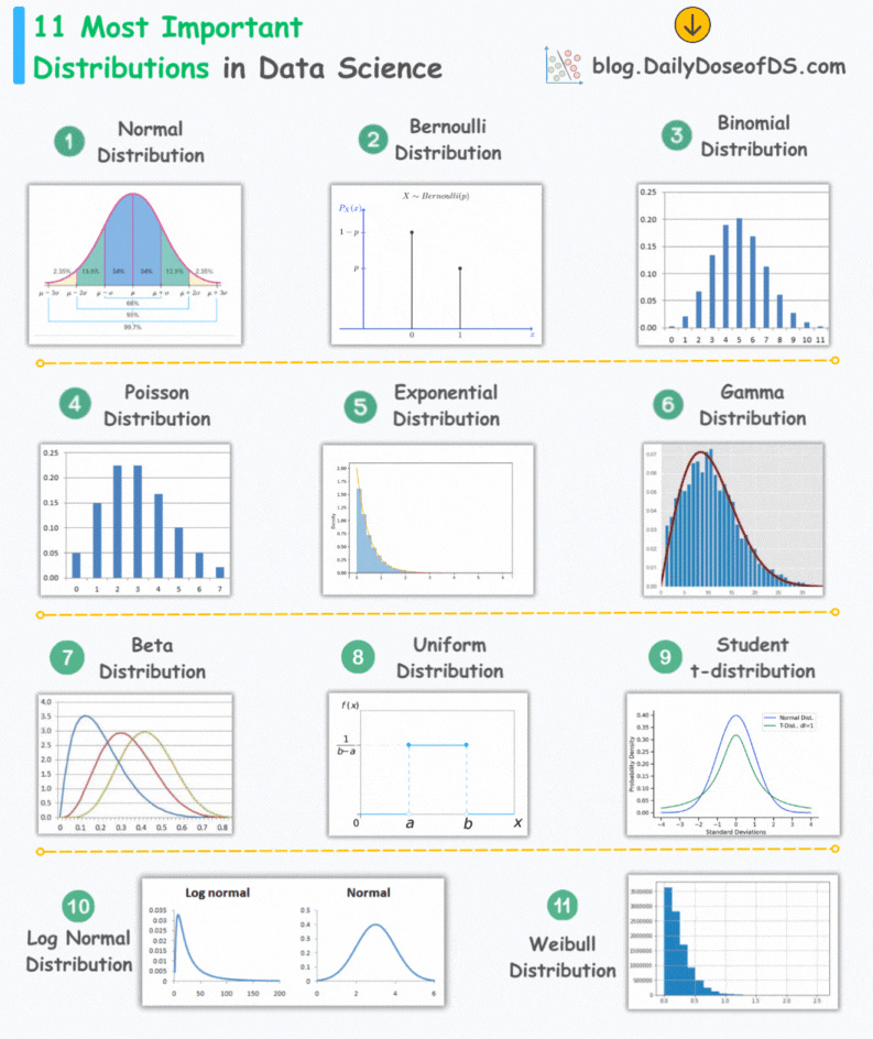
The visual below depicts the 11 most important distributions in data science:

Today, let’s understand them briefly and how they are used.

Normal Distribution
Normal distribution PDF
- The most widely used distribution in data science.
- Characterized by a symmetric bell-shaped curve
- It is parameterized by two parameters—mean and standard deviation.
- Example: Height of individuals.
Bernoulli Distribution
Bernouilli PDF
- A discrete probability distribution that models the outcome of a binary event.
- It is parameterized by one parameter—the probability of success.
- Example: Modeling the outcome of a single coin flip.
Binomial Distribution
Binomial Distribution PDF
- It is Bernoulli distribution repeated multiple times.
- A discrete probability distribution that represents the number of successes in a fixed number of independent Bernoulli trials.
- It is parameterized by two parameters—the number of trials and the probability of success.
Poisson Distribution
Poisson Distribution PDF
- A discrete probability distribution that models the number of events occurring in a fixed interval of time or space.
- It is parameterized by one parameter—lambda, the rate of occurrence.
- Example: Analyzing the number of goals a team will score during a specific time period.
Exponential Distribution
Exponential Distribution PDF
- A continuous probability distribution that models the time between events occurring in a Poisson process.
- It is parameterized by one parameter—lambda, the average rate of events.
- Example: Analyzing the time between goals scored by a team.
Gamma Distribution
Gamma Distribution PDF
- It is a variation of the exponential distribution.
- A continuous probability distribution that models the waiting time for a specified number of events in a Poisson process.
- It is parameterized by two parameters—alpha (shape) and beta (rate).
- Example: Analysing the time it would take for a team to score, say, three goals.
Beta Distribution
Beta Distribution PDF
- It is used to model probabilities, thus, it is bounded between [0,1].
- Differs from Binomial in this respect that in Binomial, probability is a parameter.
- But in Beta, the probability is a random variable.
Uniform Distribution
Uniform Distribution PDF
- All outcomes within a given range are equally likely.
- It can be continuous or discrete.
- It is parameterized by two parameters: a (minimum value) and b (maximum value).
- Example: Simulating the roll of a fair six-sided die, where each outcome (1, 2, 3, 4, 5, 6) has an equal probability.
Log-Normal Distribution
Log-Normal Distribution PDF
- A continuous probability distribution where the logarithm of the variable follows a normal distribution.
- It is parameterized by two parameters—mean and standard deviation.
- Example: Typically, in stock returns, the natural logarithm follows a normal distribution.
Student t-distribution
- It is similar to normal distribution but with longer tails (shown above).
- It is used in t-SNE to model low-dimensional pairwise similarities. We covered it here: t-SNE article.
Weibull
- Models the waiting time for an event.
- Often employed to analyze time-to-failure data.