11 LLM Evaluation Methods

Must-know for AI engineers (explained visually).

Delta attention in Kimi K3 to fix growing KV cache

Kimi K3 leans on a new mechanism called delta attention that does not keep a growing KV cache.

That is how it holds a million tokens of context without the memory blowing up.

Before we can understand delta attention, we need to understand attention itself.

It is a lookup. Every token stores a key, which works like an address, and a value, which is the content at that address.

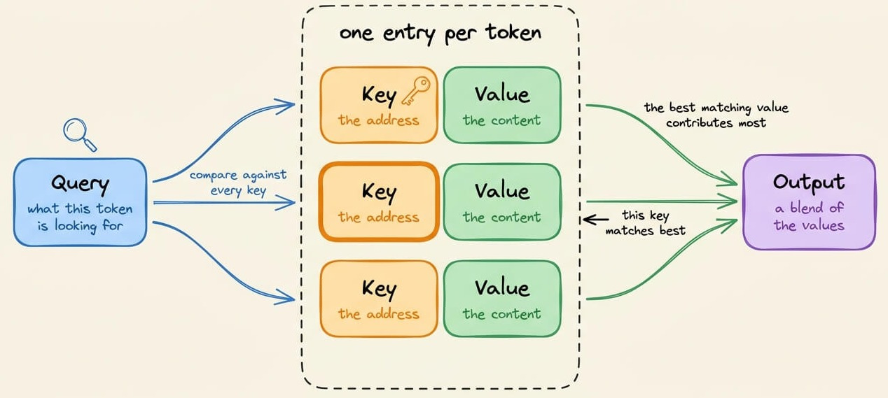
To build its output, a token sends out a query, matches it against every key in the sequence, and pulls back a blend of the values whose keys matched.

Standard attention keeps every one of those key and value pairs as a list, one entry per token.

That list is the KV cache, and it grows with the sequence, so each new token has to scan the whole thing to build its output.

Delta attention keeps the lookup process but throws away the list.

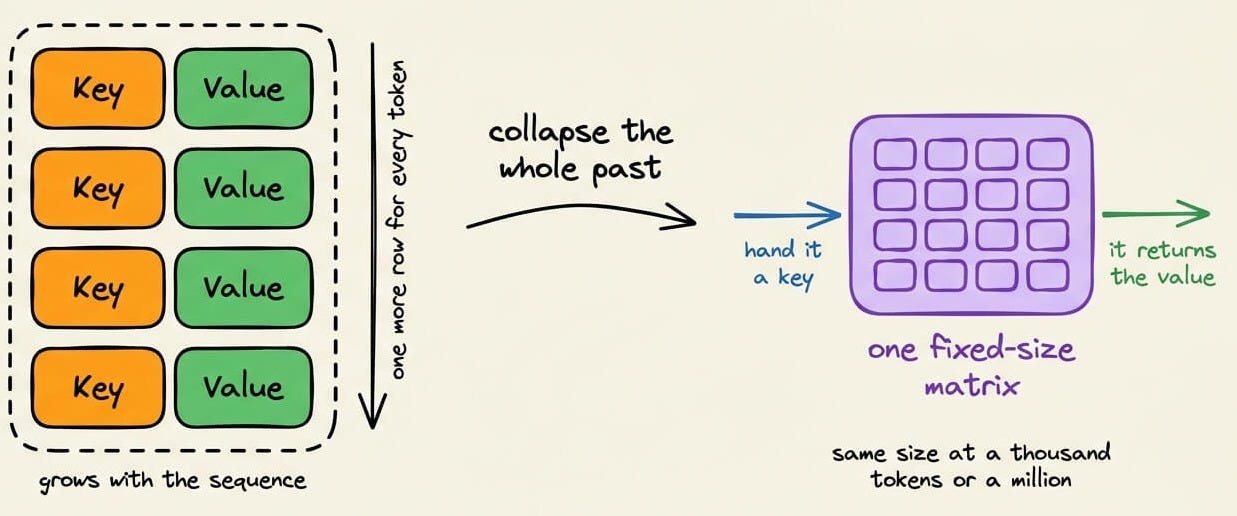
The entire past collapses into one fixed-size matrix that still behaves like the lookup table.

When you hand it a key, it returns the value vector, blended from everything the past tokens wrote, and it’s weighted by how closely each stored key matches the one you handed in.

Writing is a constrained operation. A fixed matrix has no free slot to append to, so every write lands in a direction that earlier writes already occupy and merges the two associations together.

The delta rule handles this in two moves per token, depicted below:

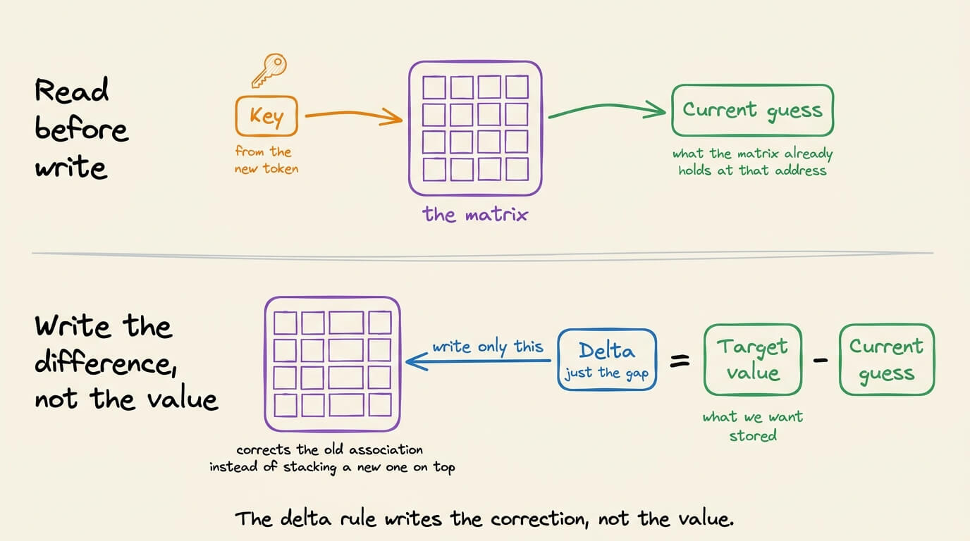
→ It reads before it writes. It hands the matrix the new token’s key and sees what value the memory currently returns, its existing guess for that address.

→ It writes the difference, not the value. It compares that guess against the value it actually wants stored and writes only the gap. That gap is the delta, and it corrects the old association instead of stacking a new one on top.

The matrix also lets old entries fade over time, so a fixed size can keep absorbing a long sequence without filling up.

Standard attention remembers by keeping everything and pays a quadratic cost to re-scan it.

Delta attention remembers by rewriting one matrix and pays a linear cost.

Of course, a compressed matrix cannot store every token exactly, so recall of any single token becomes approximate. That is why production models interleave the two, i.e., a few full-attention layers for exact lookup and the rest running linear.

Read more in the official announcement blog here →

---

11 LLM evaluation methods

A model can answer a question correctly and still score close to zero on BLEU.

That happens whenever the model says the right thing in different words than the reference. BLEU compares n-gram overlap, so a clean paraphrase reads as a total miss.

This one failure is why LLM evaluation is fragmented into several methods, depicted below:

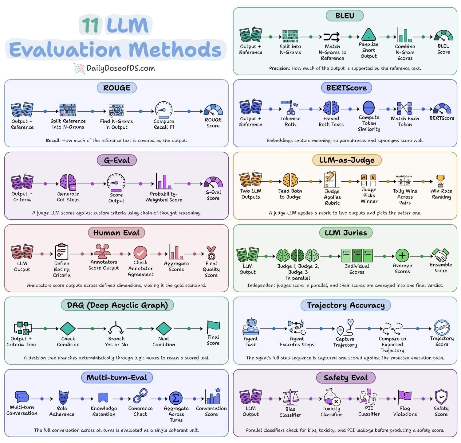
Each method encodes a different assumption about what a correct output looks like, and different metrics are useful in different use cases.

Let’s understand the 11 must-know LLM evaluation metrics below

---

1) BLEU

Splits output and reference into n-grams and measures how much of the output is supported by the reference, with a brevity penalty so short outputs cannot win by omission.

It works for translation and constrained generation where the reference wording is close to the only acceptable wording. Report corpus-level BLEU instead of averaging sentence scores, and supply multiple references when more than one phrasing is correct.

2) ROUGE

Flips the direction of BLUE and measures recall, meaning how much of the reference is covered by the output.

It is the default for summarization and extraction, where missing content hurts more than extra content. ROUGE-L uses longest common subsequence and tolerates reordering better than ROUGE-2. Recall alone rewards verbosity, so it needs a precision-side metric next to it.

3) BERTScore

Embeds both texts, matches each output token to its most similar reference token, and reports precision, recall, and F1 over those similarities.

It handles the paraphrase case that causes problems in BLEU and ROUGE. Absolute values lie within a narrow high band, so scores are only meaningful when compared across systems, not read as accuracy. Rescaling the baseline helps, and the embedding model has to match the domain and language.

4) G-Eval

It hands a task description and criteria to a judge model to generate chain-of-thought evaluation steps, then scores against those steps with the result weighted by token probabilities.

It fits subjective criteria with no reference answer, like tone, instruction following, or domain correctness. Criteria written as a concrete checklist score far more consistently than criteria written as adjectives.

Ideally, it is recommended to run the judge at a low temperature and calibrate against a small human-labeled set before trusting it.

5) LLM-as-Judge

The pairwise form feeds two or more outputs to a judge with a rubric, the judge picks the better one:

It is the practical way to compare two models, two prompts, or two retrieval configs when absolute scores drift between runs.

Make sure to randomize which output appears first, because judges might favor a position. You also need to control for length, since judges reliably prefer longer answers regardless of quality.

6) Human eval

Annotators score outputs across defined dimensions, and the aggregate becomes the reference that every automated metric gets calibrated against.

It belongs in two places, building the calibration set that validates a judge, and the final gate before release.

You must define the rubric before annotation starts and measure inter-annotator agreement. Low agreement means the rubric is ambiguous, not that the annotators are wrong.

7) LLM juries

Runs several judges independently over the same output and averages their scores into one verdict.

It exists because a single judge carries a stable bias, including a preference for outputs from its own model family.

Use different model families rather than the same model three times, since correlated judges average away noise but not bias. Several small models in a jury often beat one large judge at a lower cost.

8) DAG

Scores through a decision tree where each node asks one narrow question and the answer routes to the next node, with the final leaf carrying the score.

It fits rubrics with hard requirements and ordering, like format compliance, required sections, or a mandatory disclaimer.

Because branching is deterministic, the same output always gets the same score. Always put cheap deterministic checks near the root so failing outputs exit before any model call.

9) Trajectory accuracy

Captures the agent’s full sequence of thoughts, tool calls and observations, then scores that path against the expected one.

It matters because an agent can reach the right answer through the wrong path, burning tokens on redundant calls or touching a tool it should not have.

Score path and outcome separately, otherwise a lucky correct answer hides a broken execution path. This needs tracing in place first, since there is no trajectory to score without it.

10) Multi-turn eval

Treats the whole conversation as the unit and scores role adherence, knowledge retention across turns, and coherence.

Per-turn scoring misses the failures that only appear over time, like contradicting an earlier answer or dropping a constraint set five turns ago.

Run it on real conversation logs rather than synthetic two-turn exchanges, because rule retention failures show up at depth.

11) Safety eval

Runs bias, toxicity and PII classifiers in parallel over the output and flags violations instead of producing a quality score.

It belongs as a gate, not as a term inside an average. A single PII leak matters regardless of how good the mean quality score looks, which is how folding safety into an aggregate ends up shipping violations.

---

To use them in practice, most of these already ship as built-in metrics in Comet Opik, an open-source LLM evaluation and observability platform, including BLEU, ROUGE, BERTScore, G-Eval, LLM juries, trajectory accuracy, conversation-level metrics, and moderation, all running over traced production data.

Here’s the repo → https://github.com/comet-ml/opik

(don’t forget to star it ⭐️)

Also, to dive deeper in the full LLMOps lifecycle, we have covered every bit of it in the LLMOps course, starting from fundamentals to productions:

• Read Part 1 on fundamentals of LLMOps here →

• Read Part 2 on understanding the core building blocks of LLMs →

• Read Part 3 on the key components of LLMs, focusing on the attention mechanism, architectures like transformers and mixture-of-experts, and the fundamentals of pretraining and fine-tuning →

• Read Part 4 on decoding strategies, generation parameters, best practices, and the broader lifecycle of LLM-based applications →

• Read Part 5 on context + prompt engineering from a system perspective, in-context learning, types of prompts, and different prompting techniques →

• Read Part 6 on prompt versioning, defensive prompting, and techniques like verbalized sampling, role prompting, and more →

• Read Part 7 on context engineering, covering context types, context construction principles, and retrieval-centric techniques for building high-signal inputs →

• Read Part 8 on memory, dynamic, and temporal context in LLM systems, covering short and long-term memory, dynamic context injection, and common failure modes in agentic applications →

• Read Part 9 on evaluation methods and approaches for LLM-based applications, primarily focusing on building a strong understanding of the fundamental concepts →

• Read Part 10 on evaluation benchmarks in LLM applications, with task-specific methodologies, and the core tooling for evaluation of LLM apps →

• Read Part 11 on evaluation of multi-turn systems, tool use evaluations, tracing, and red teaming →

• Read Part 12 on LLM fine-tuning, parameter-efficient methods like LoRA and QLoRA, and alignment techniques such as RLHF, DPO, and GRPO →

• Read Part 13 on LLM inference optimization, KV caching, PagedAttention, FlashAttention, speculative decoding, and model parallelism →

• Read Part 14 on the fundamentals of LLM serving, including API-based access, inference with vLLM, and practical decisions.

👉 Over to you: What else would you add to the master tree?

Good day!