11 Powerful Techniques to Supercharge Your ML Models
Take your ML models to the next level.
Many ML engineers quickly pivot to building a different model when they don't get satisfying results with one kind of model.
They do not fully exploit the possibilities of existing models and continue to move towards complex ones.
But after building so many ML models, I have learned various techniques that uncover nuances and optimizations we could apply to significantly enhance model performance without necessarily increasing the model complexity.
I have put together 11 such high-utility techniques in a recent article here: 11 Powerful Techniques To Supercharge Your ML Models.
The article provides the clear motivation behind their usage, as well as the corresponding code, so that you can start using them right away.
Let’s discuss one of them below.
The issue with regression models
A big problem with most regression models is that they are sensitive to outliers.
Consider linear regression, for instance.
Even a few outliers can significantly impact Linear Regression performance, as shown below:
And it isn’t hard to identify the cause of this problem.
Essentially, the loss function (MSE) scales quickly with the residual term (true-predicted).
Thus, even a few data points with a large residual can impact parameter estimation.
Huber Regression
Huber loss (or Huber Regression) precisely addresses this problem.
In a gist, it attempts to reduce the error contribution of data points with large residuals.
How?
One simple, intuitive, and obvious way to do this is by applying a threshold (δ) on the residual term:
If the residual is smaller than the threshold, use MSE (no change here).
Otherwise, use a loss function that has a smaller output than MSE — linear, for instance.
This is depicted below:
For residuals smaller than the threshold (δ) → we use MSE.
Otherwise, we use a linear loss function which has a smaller output than MSE.
Mathematically, Huber loss is defined as follows:
Its effectiveness is evident from the image below:
Linear Regression is affected by outliers
Huber Regression is more robust.
Now, I know what you are thinking.
How do we determine the threshold (δ)?
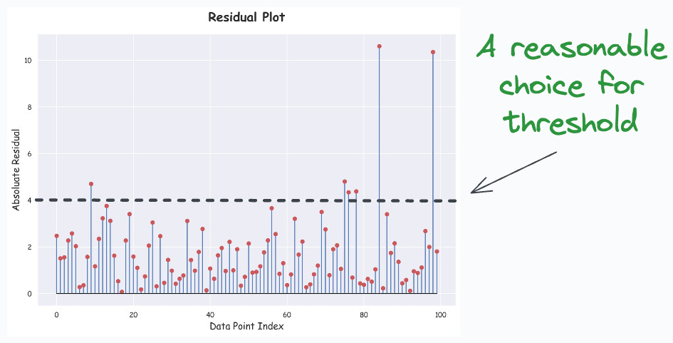
While trial and error is one way, I often like to create a residual plot. This is depicted below:
The below plot is generally called a lollipop plot because of its appearance.
Train a linear regression model as you usually would.
Compute the residuals (=true-predicted) on the training data.
Plot the absolute residuals for every data point.
One good thing is that we can create this plot for any dimensional dataset. The objective is just to plot (true-predicted) values, which will always be 1D.
Next, you can subjectively decide a reasonable threshold value δ.
See…that was so simple and profound, wasn’t it?
Check out the full article where I have put together 11 such high-utility techniques: 11 Powerful Techniques To Supercharge Your ML Models.
The article provides the clear motivation behind their usage, as well as the corresponding code, so that you can start using them right away.
Thanks for reading!


