

In today’s newsletter:
Build voice agents that hear the details.
16 policy optimization methods for LLM training.
How hybrid LLMs shrink the KV cache, explained visually.
Build voice agents that hear the details
Speechmatics Linden is a speech-to-text model built specifically for voice agents. It focuses on the inputs that tend to cause expensive mistakes: strong accents, background noise, non-native speech, names, and alphanumeric strings such as booking references.

Real-time transcription across 55+ languages
Final transcripts in roughly 250 ms after a
ForceEndOfUtterancesignalCustom dictionaries for names, product terms, and industry vocabulary
Native integrations for LiveKit, Pipecat, Jambonz, and the Speechmatics API
Linden 1 costs $0.30 per hour for new users, with volume discounts bringing the price down to $0.16 per hour
New accounts receive $100 in credit with no card required, which covers roughly 333 hours of Linden 1 transcription at the standard $0.30 per-hour rate.
Thanks to Speechmatics for partnering today!
16 policy optimization methods for LLM training
The fastest way to make LLM RL cheaper is to delete a model.
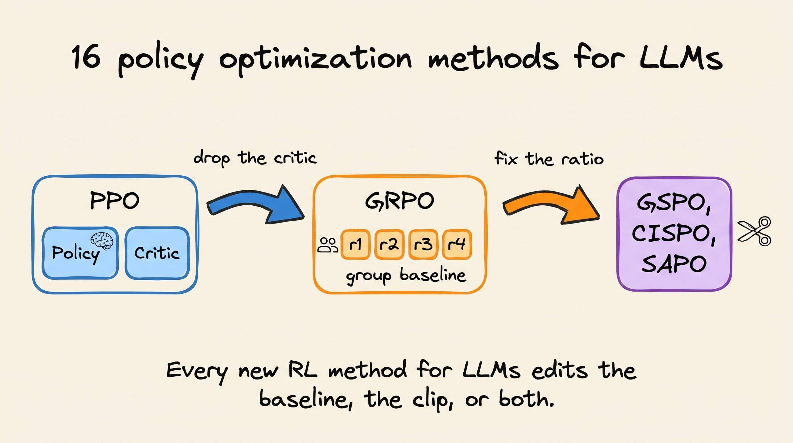
ReMax did exactly that in 2023. It dropped PPO’s value model and cut GPU memory by about 46% when training a 7B model.
Most of the methods below make a similar trade. They remove a component, or they change how far a single update can move the policy.
The visual below maps 16 of them.
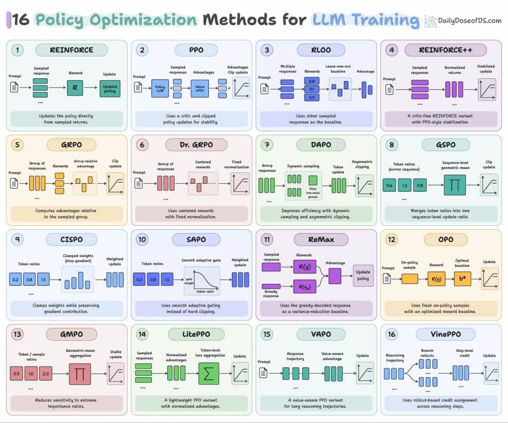
Under the hood, all 16 run the same loop. We sample responses from the current policy and score them with a reward model or a verifier. Then we compute an advantage, which says how much better a response was than expected, and update the policy.
The update weights each token by an importance ratio, the new policy’s probability divided by the old one’s. PPO-style methods clip that ratio so one batch can’t drag the policy too far.
So every method answers two questions. What do we compare the reward against, and what do we do with ratios that drift too far?
Grouping them by those answers gives four families.
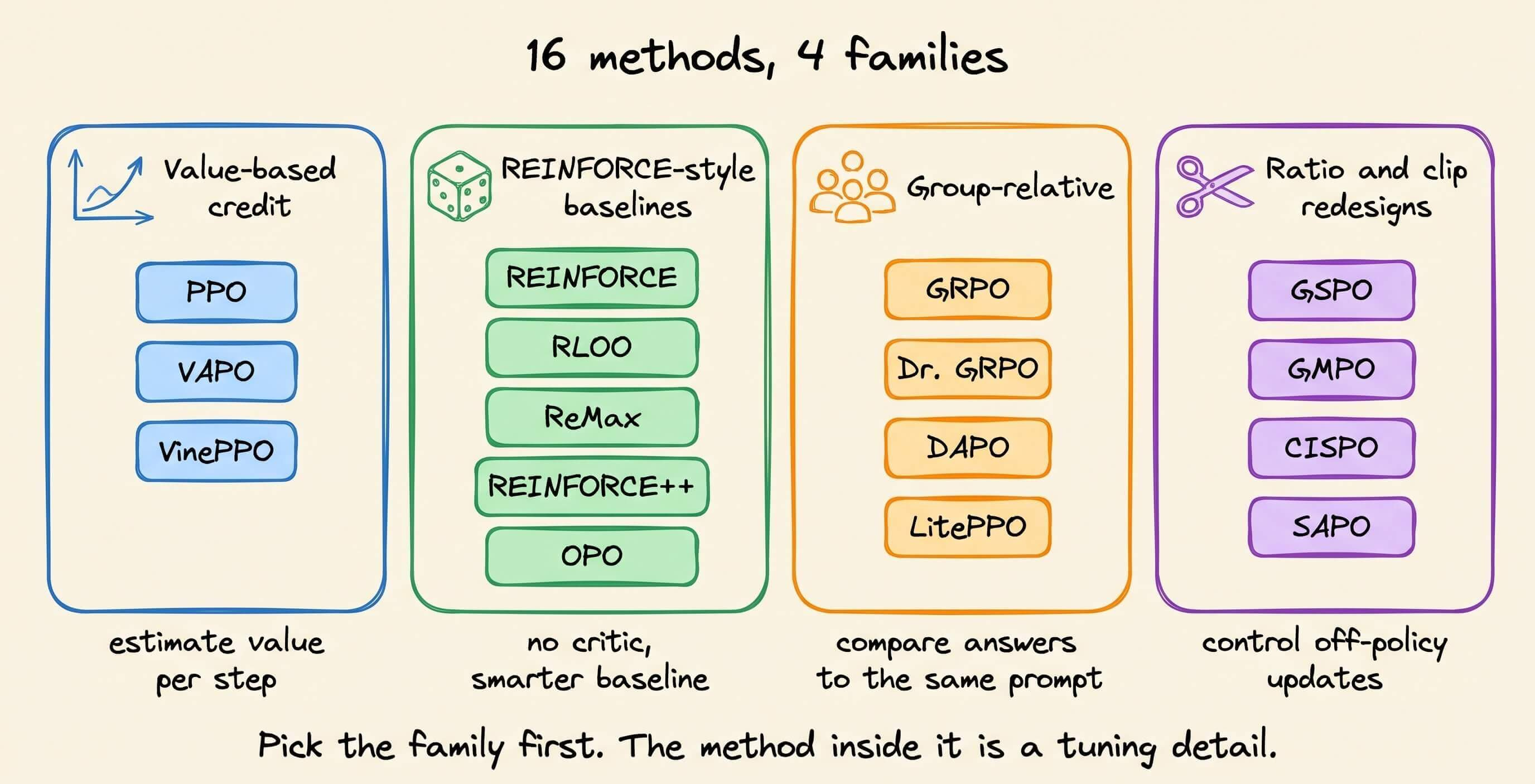
Value-based credit: PPO, VAPO, VinePPO
PPO clips the token ratio, typically to the range 0.8 to 1.2. In RLHF, it also trains a critic that predicts the expected reward at every token, and GAE turns those predictions into per-token advantages.
The critic is expensive and it isn’t always accurate. The VinePPO authors found that value networks on reasoning tasks often estimate returns poorly and barely beat a random baseline when ranking alternative steps.
VAPO keeps the critic and repairs it for long chains of thought. It pretrains the value model against a fixed policy, decouples GAE between the actor and the critic, and adapts GAE’s λ to response length. Built on a Qwen 32B base model, it reported 60.4 on AIME 2024 within 5,000 steps.
VinePPO removes the value network instead. A language environment can restart from any partial answer by re-feeding the prefix, so VinePPO runs extra rollouts from intermediate steps and averages their rewards. That gives an unbiased Monte Carlo value for each step.
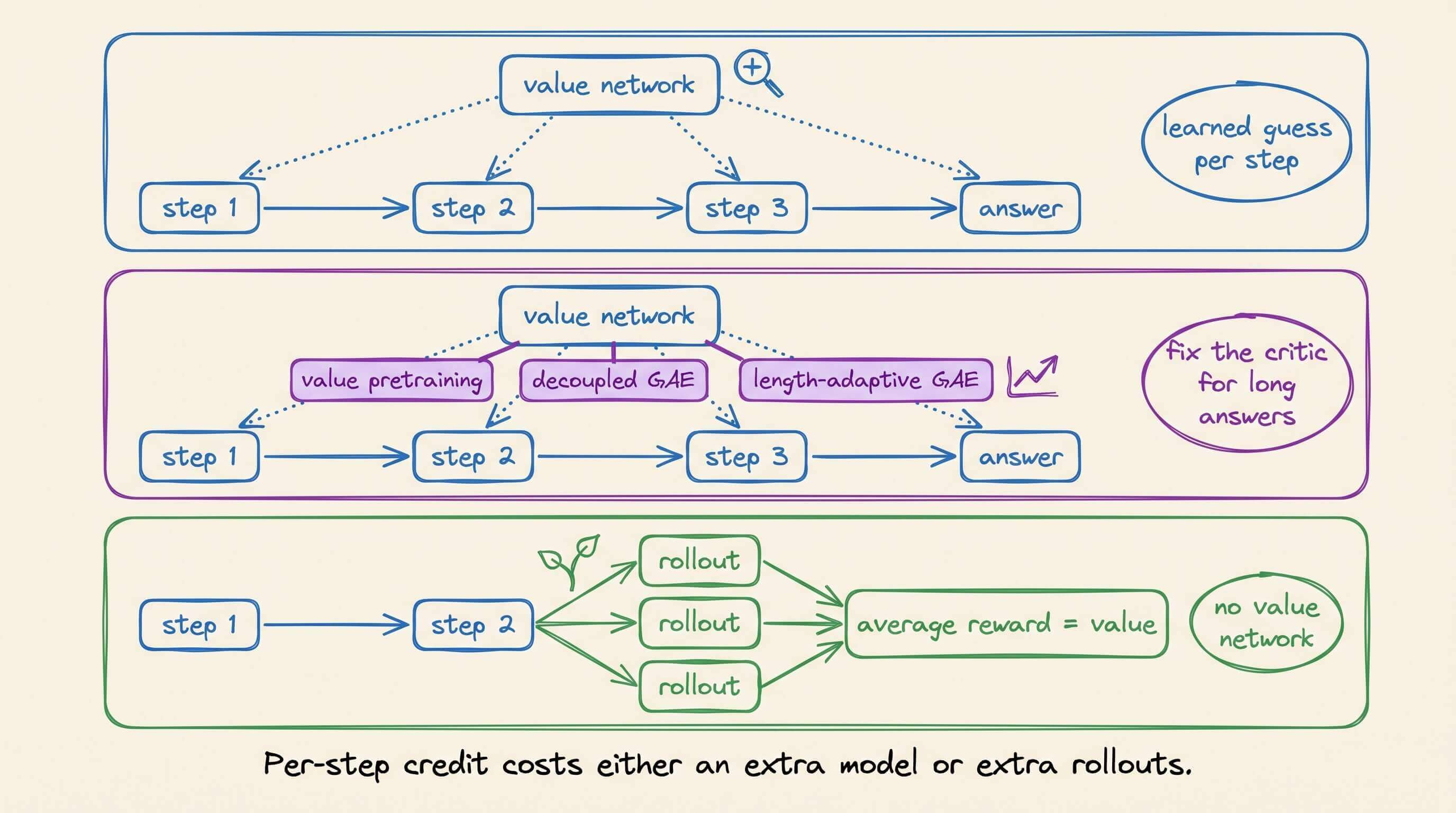
On MATH and GSM8K, VinePPO beat PPO in up to 3x less wall-clock time.
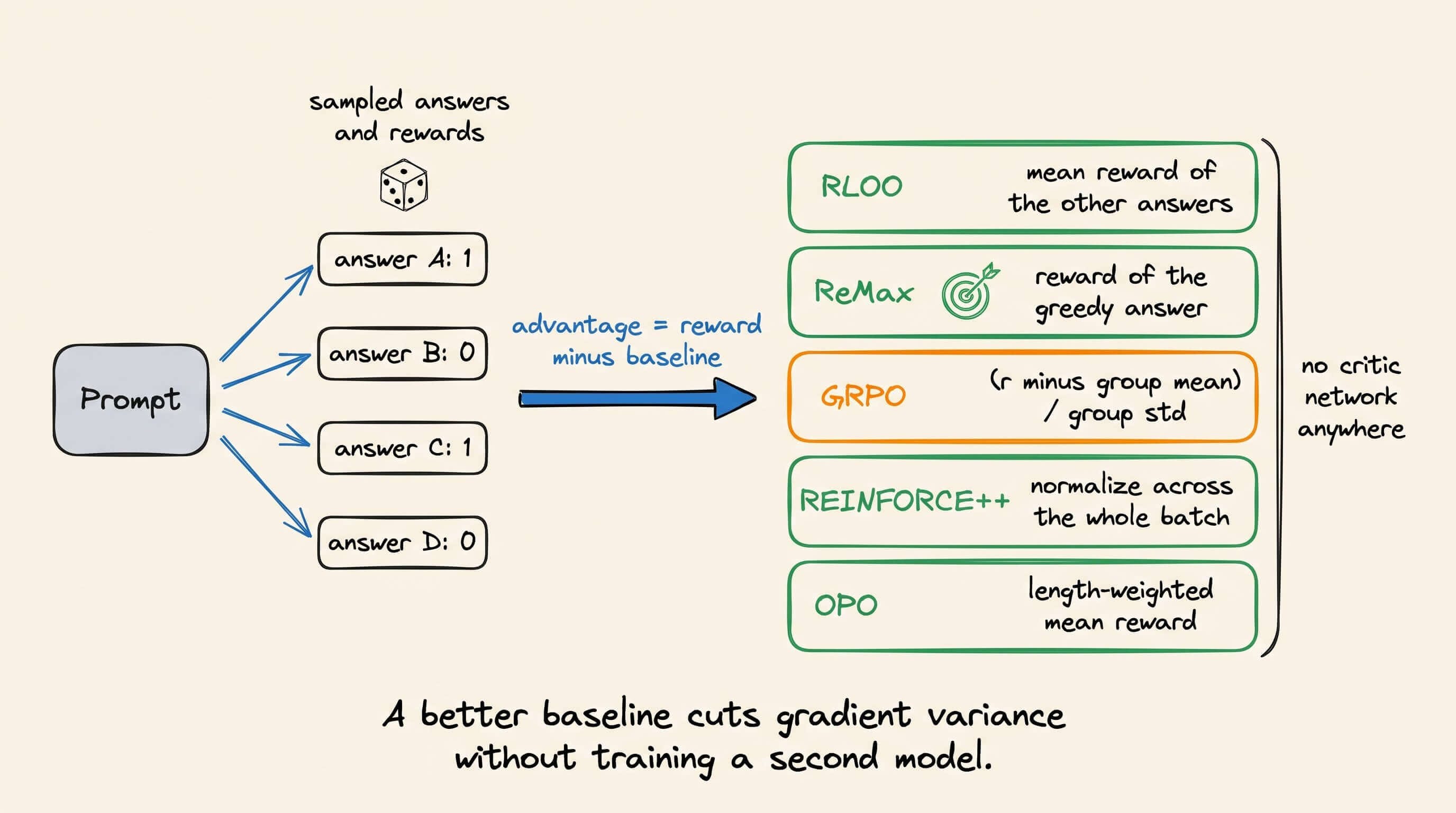
REINFORCE-style baselines: REINFORCE, RLOO, ReMax, REINFORCE++, OPO
These methods skip the critic and treat the whole response as one action with one reward. The design question becomes what to subtract from that reward.
REINFORCE is the plain policy gradient from 1992. It raises the log-probability of a sampled response in proportion to its reward, optionally minus a baseline.
RLOO samples k responses per prompt and uses the mean reward of the other k-1 responses as each one’s baseline. Cohere’s 2024 study showed REINFORCE-style methods like this outperform PPO, DPO, and RAFT in RLHF.
ReMax uses the reward of the greedy-decoded response as the baseline. One extra greedy generation replaces an entire value network.
REINFORCE++ normalizes advantages across the entire global batch instead of within each prompt’s group. Its authors show prompt-level normalization is biased, while the global version’s bias vanishes as the batch grows.
OPO enforces exact on-policy training and derives the baseline that minimizes gradient variance. Under a simplifying assumption, that baseline becomes a length-weighted mean of rewards, so longer responses count more.
OPO needs no value model, no reference model, and no KL term. Its implementation is merged into verl.
Group-relative: GRPO, Dr. GRPO, DAPO, LitePPO
GRPO came from DeepSeekMath. It samples a group of responses per prompt, normalizes each reward by the group’s mean and standard deviation, and feeds that advantage into PPO’s clipped objective with a KL penalty to a reference model.
There’s no critic, and DeepSeek later used GRPO to train DeepSeek-R1. But its defaults carry biases.
Dr. GRPO shows that GRPO’s per-response length normalization pushes response length up, especially for wrong answers. It removes both the length and the standard-deviation normalization terms. With it, the authors’ 7B recipe reached 43.3% on AIME 2024.
DAPO from ByteDance Seed makes four changes and also drops the KL term:
Clip-Higher decouples the clip range to 0.2 below and 0.28 above, so low-probability exploration tokens can grow.
Dynamic Sampling over-samples and filters out prompts where every answer is right or every answer is wrong, since those groups produce zero advantage.
A token-level loss weights long responses by their token count.
Overlong reward shaping applies a soft, length-aware penalty to responses that run past the length limit.
DAPO reached 50 points on AIME 2024 with a Qwen2.5-32B base model.
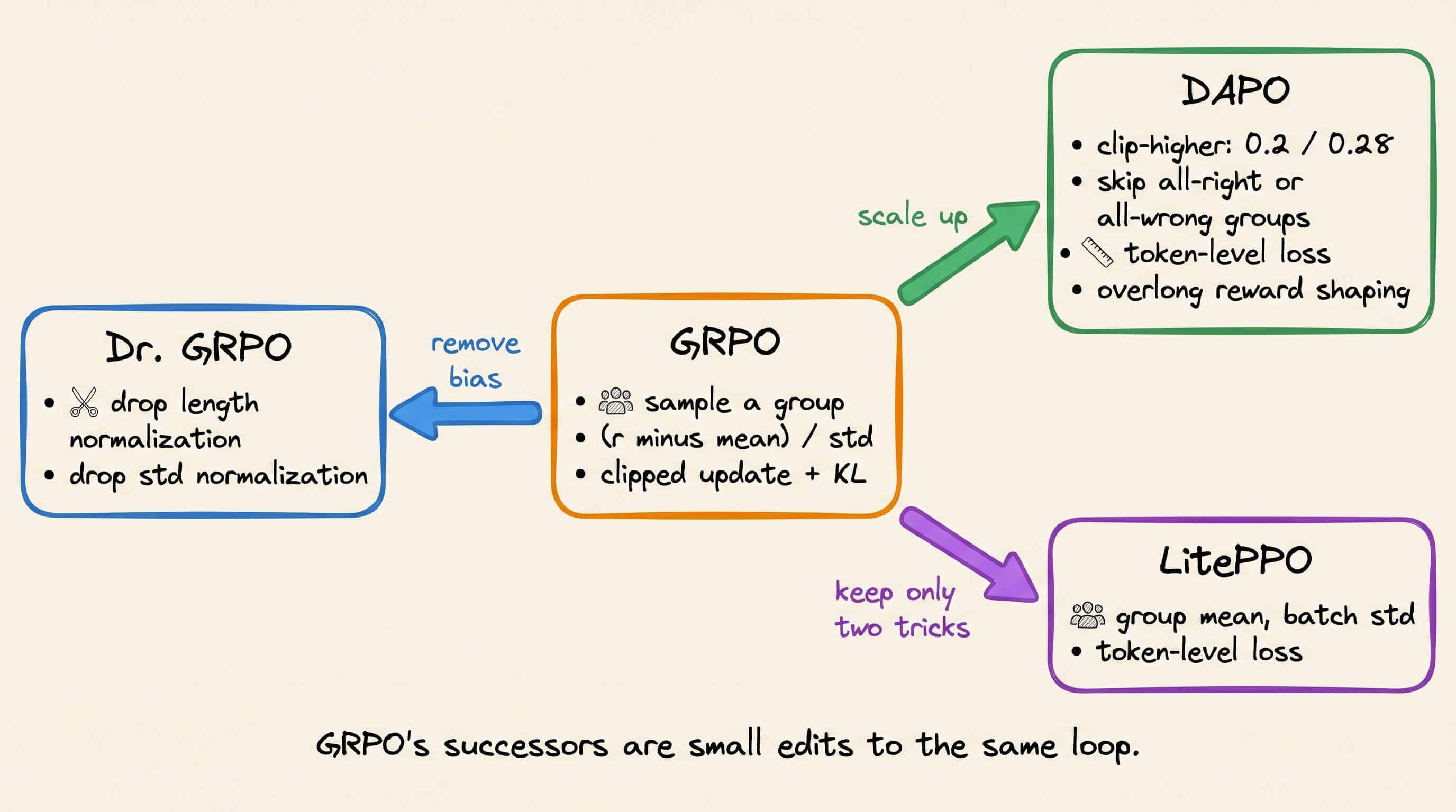
LitePPO tested these tricks one at a time. It kept only two: group-level mean with batch-level standard deviation for the advantage, and token-level loss aggregation, on a vanilla PPO loss without a critic. In the authors’ experiments, that pair beat both GRPO and DAPO.
Ratio and clipping redesigns: GSPO, GMPO, CISPO, SAPO
Every method above reuses samples from a slightly older policy, so the token ratios drift. The SAPO authors note that this variance gets worse in Mixture-of-Experts models.
GSPO from Qwen computes one ratio per sequence, the length-normalized sequence likelihood ratio, which works out to the geometric mean of the token ratios. Clipping happens at the sequence level. The Qwen team reports that it stabilizes MoE RL training and credits it with gains in Qwen3.
GMPO maximizes the geometric mean of the token-level objectives instead of the arithmetic mean, so one outlier ratio can’t dominate. It stays stable with a clip range of e^-0.4 to e^0.4, wider than GRPO’s 0.8 to 1.2, and improved GRPO’s average Pass@1 by up to 4.1% at 7B.
CISPO comes from the MiniMax-M1 report. It clips the importance-sampling weight and stops the gradient through it, instead of clipping the token update. Every token still contributes a gradient, and in a Qwen2.5-32B study it matched DAPO’s AIME score in half the training steps.
SAPO, also from Qwen, replaces the hard clip with a smooth, temperature-controlled gate. When a few tokens in a sequence go off-policy, GSPO suppresses the gradient for the whole sequence. SAPO down-weights only those tokens. Qwen used it to train the Qwen3-VL series.
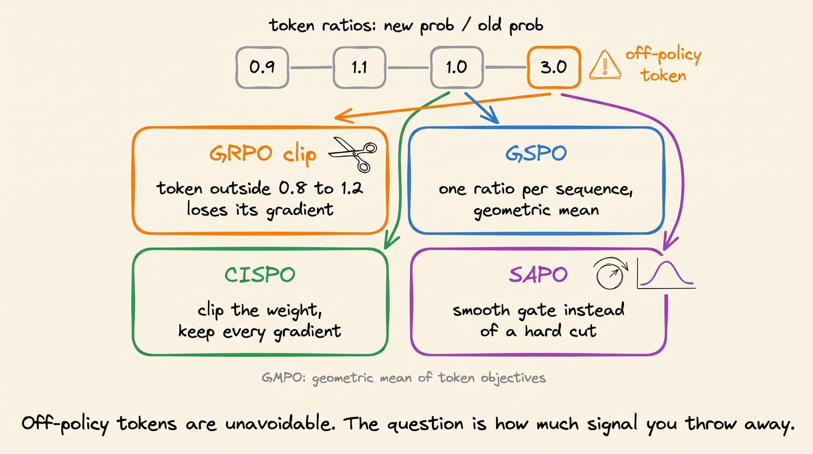
Laid out this way, the 16 names collapse into two dials: the baseline and the clip.
When the next RL paper lands, check which of the two it touches first. That usually tells you whether it fixes a problem you actually have.
If you want to understand where these dials come from, our RL course builds them from scratch, from the Bellman equations to REINFORCE, PPO, RLHF, GRPO, and agentic RL:
👉 Over to you: Which policy optimization method runs in your post-training stack today?
How hybrid LLMs shrink the KV cache
Every attention layer stores a key and a value for every token it has seen.
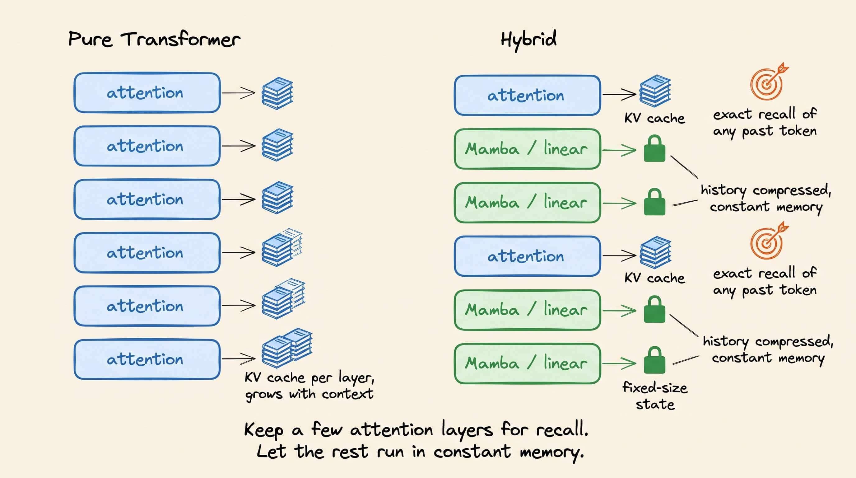
Hybrid LLMs keep only a few attention layers. The rest are linear-attention or state-space layers, like Mamba, that compress everything seen so far into a fixed-size state.
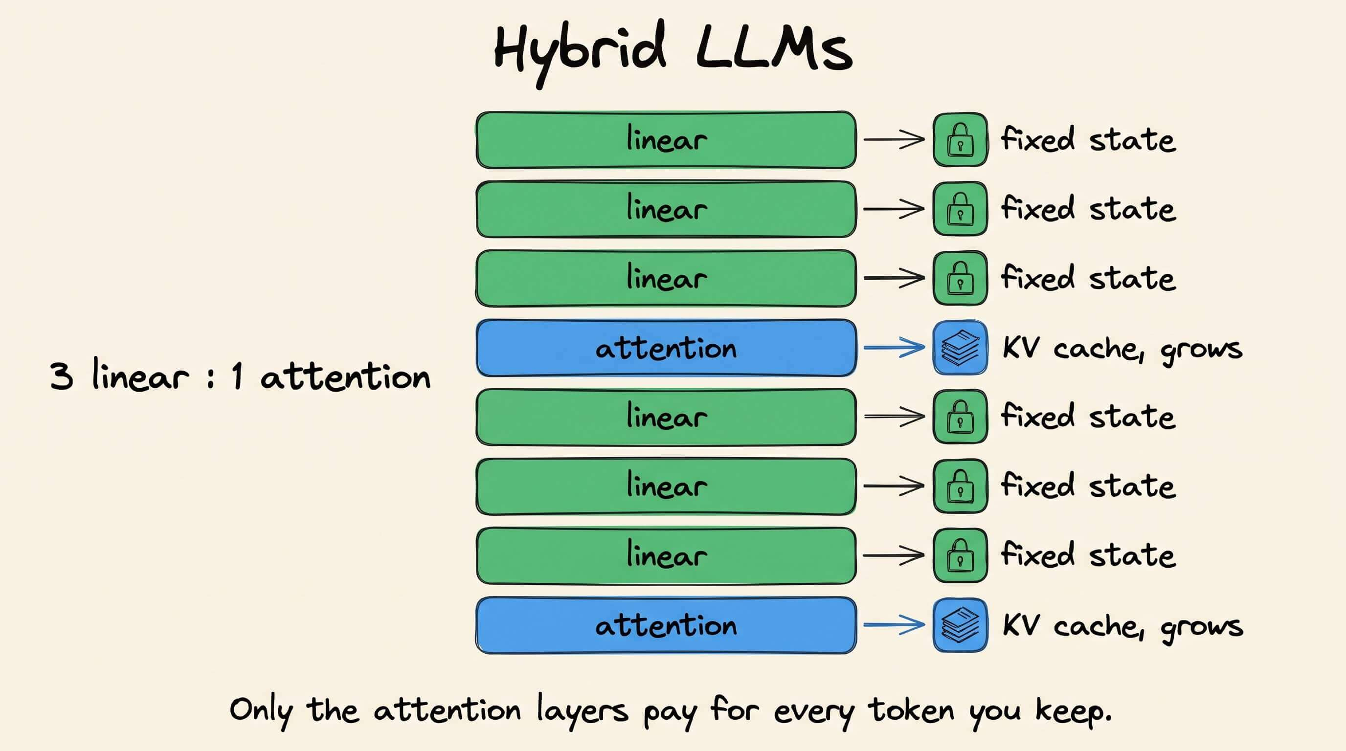
That state does not grow with context. The visual below shows the difference on one 262K-token sequence.
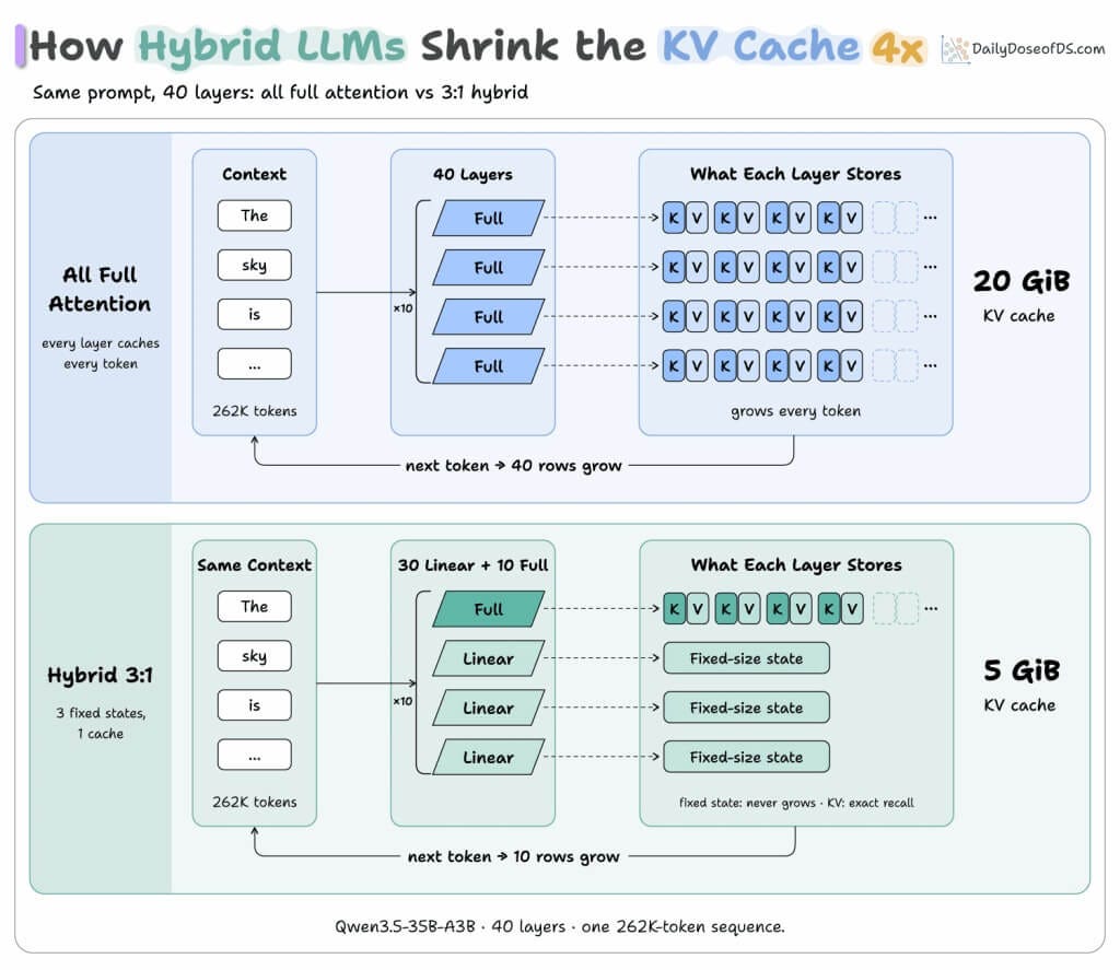
Qwen3.5-35B-A3B has 40 layers, laid out as 10 repeats of three Gated DeltaNet layers followed by one gated attention layer. Only those 10 attention layers write to the KV cache.
Each attention layer caches 2 KV heads of 256 dimensions for keys and values. At 16 bits, that is 2,048 bytes per token per layer, or 512 MiB per layer at 262,144 tokens.
40 layers give 20 GiB.
10 layers result in 5 GiB.
Each Gated DeltaNet layer instead carries a recurrent state of 32 heads × 128 × 128 values, whether the context is 1K tokens or 262K.
So why not do fully linear?
A fixed-size state is lossy.
When AI21 built Jamba, a pure Mamba model struggled with in-context learning, for example, following the output format shown in few-shot examples, while the attention-Mamba hybrid behaved like a vanilla Transformer.
Attention layers are where exact recall of any past token lives. Hybrids keep a few of them and let the rest run in constant memory.
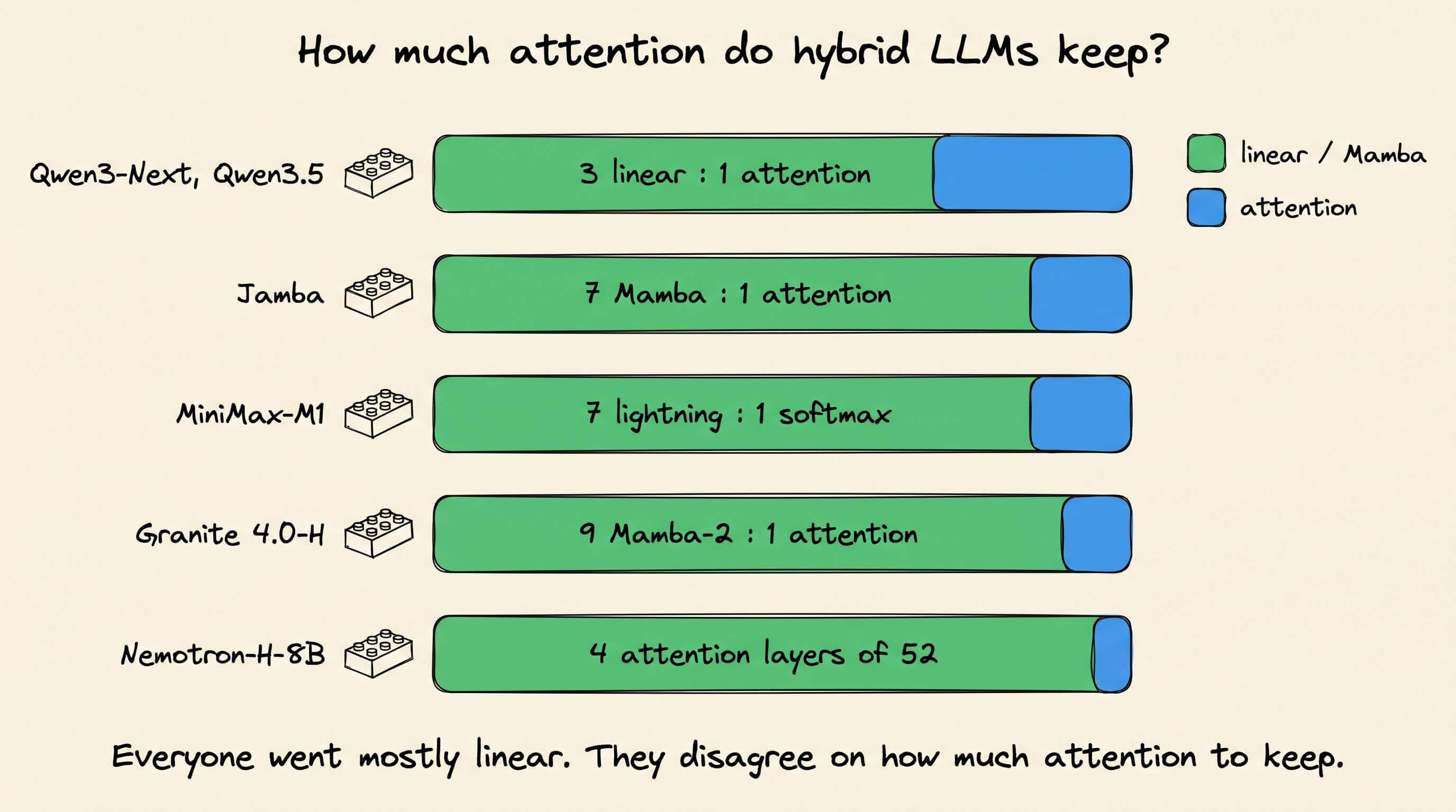
Labs have converged on mostly linear stacks but disagree on how much attention to keep:
↳ Qwen3-Next-80B-A3B and Qwen3.5 → 3 Gated DeltaNet layers per gated attention layer. Qwen reports that Qwen3-Next-80B-A3B gets 10x the inference throughput of Qwen3-32B for contexts over 32K tokens.
↳ Jamba → 1 attention layer per 7 Mamba layers. Its KV cache at 256K tokens is 4GB, versus 32GB for Mixtral.
↳ MiniMax-M1 → 1 softmax attention block after every 7 lightning attention blocks. At a 100K-token generation length, it uses about 25% of DeepSeek R1’s FLOPs.
↳ Granite 4.0-H → 9 Mamba-2 blocks per transformer block. IBM reports over 70% less RAM for long inputs and concurrent batches.
↳ Nemotron-H → roughly 8% attention layers, 4 of 52 in the 8B model and 10 of 118 in the 56B model. NVIDIA reports up to 3x faster inference than similarly sized Transformers.
This ties back to the main section, too. MiniMax trained M1 with CISPO, and its report credits the hybrid attention design plus CISPO for finishing full RL training on 512 H800 GPUs in three weeks.
The savings grow with context length and concurrency. At short contexts, the KV cache is small anyway, and the real speedup depends on how well your serving engine implements the linear layers. The Qwen3-Next model card itself notes that the throughput gain “depends highly on the implementation.”
Hybrid layers are one of 12 ways to shrink the KV cache. We covered all of them in our KV cache engineering article, including GQA, multi-head latent attention, sliding windows, quantization, eviction, paging, prefix reuse, and offloading, plus how to combine them.
Read the KV cache engineering article here →
Good day!