5 Embedding Compression Techniques

...explained visually.

The easiest way to find out which models you can run on your computer:

Just run:

npm i -g @magnitudedev/cli
magnitude setup

It profiles your machine and ranks the models across:

• Speed

• Accuracy

• Intelligence

• Memory required

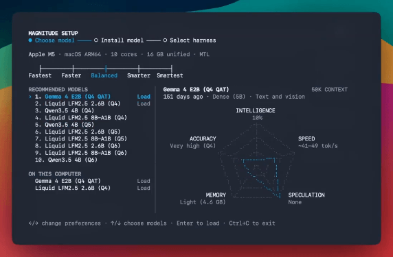
Finally, you can choose your favorite harness (Pi, OpenCode, Claude Code, Codex, etc.) to run with it.

Here’s the GitHub repo →

(don’t forget to star 🌟)

---

5 embedding compression techniques

Ten million 1,536-dimensional embeddings will occupy:

• 62 GB in float32

• 15 GB in int8

• 2 GB as packed bits

This only covers the raw vector payload, and an in-memory system also needs space for the ANN index, metadata, and allocator overhead.

Embedding compression works along two axes:

• the number of dimensions stored

• the number of bits used for each dimension

The five techniques in the visual reduce different parts of the payload.

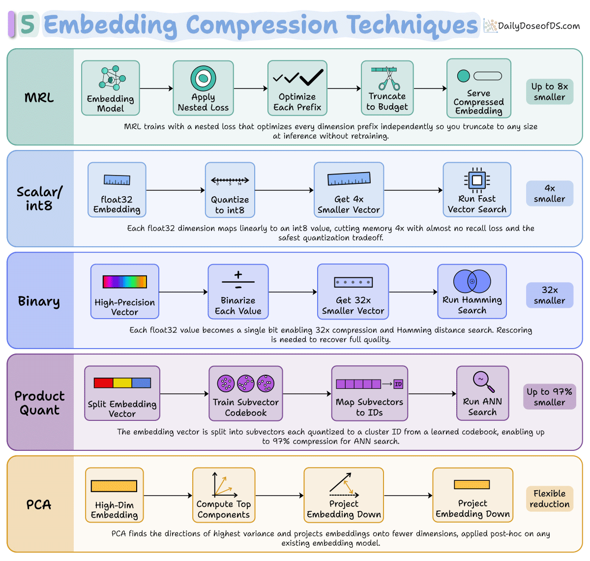
1) PCA applies a post-training transform:

It learns the directions with the most variance from a representative sample, then projects existing embeddings into a smaller space.

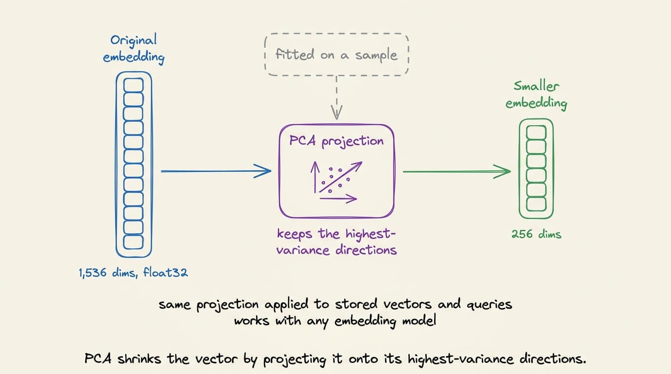
It works with any embedding model, although the projection must be fitted and applied consistently to indexed vectors and queries.

2) MRL alters the training objective:

The model is trained so that selected prefixes (say, the first <n> dimensions) of the embedding remain useful independently.

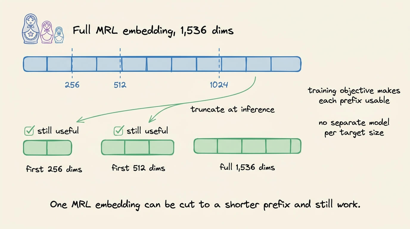
You can therefore truncate an MRL embedding at inference without training a separate model for every target dimension.

OpenAI reports that text-embedding-3-large at 256 dimensions still outperforms the 1,536-dimensional text-embedding-ada-002 on MTEB.

3-4) Scalar and binary quantization keep the dimension count fixed and reduce the representation used for each value.

Scalar quantization typically maps float32 values to int8, giving a 4x reduction in the raw vector payload.

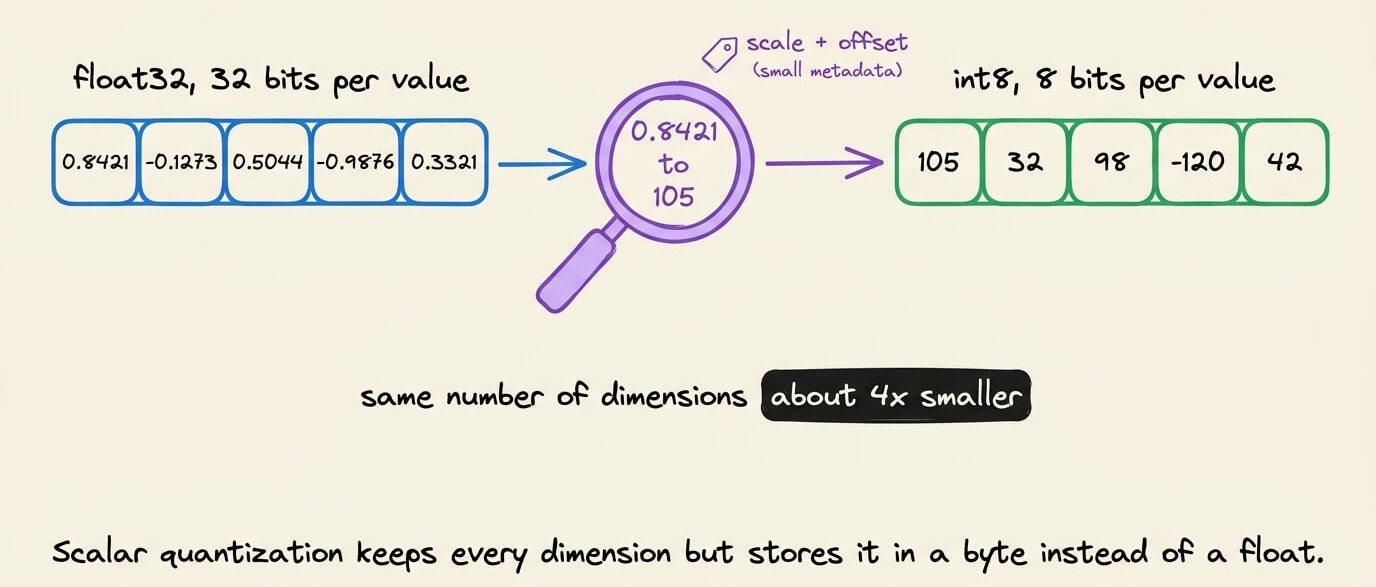
The scale and offset add a small amount of metadata.

Binary quantization keeps one bit per dimension, which gives a 32x reduction.

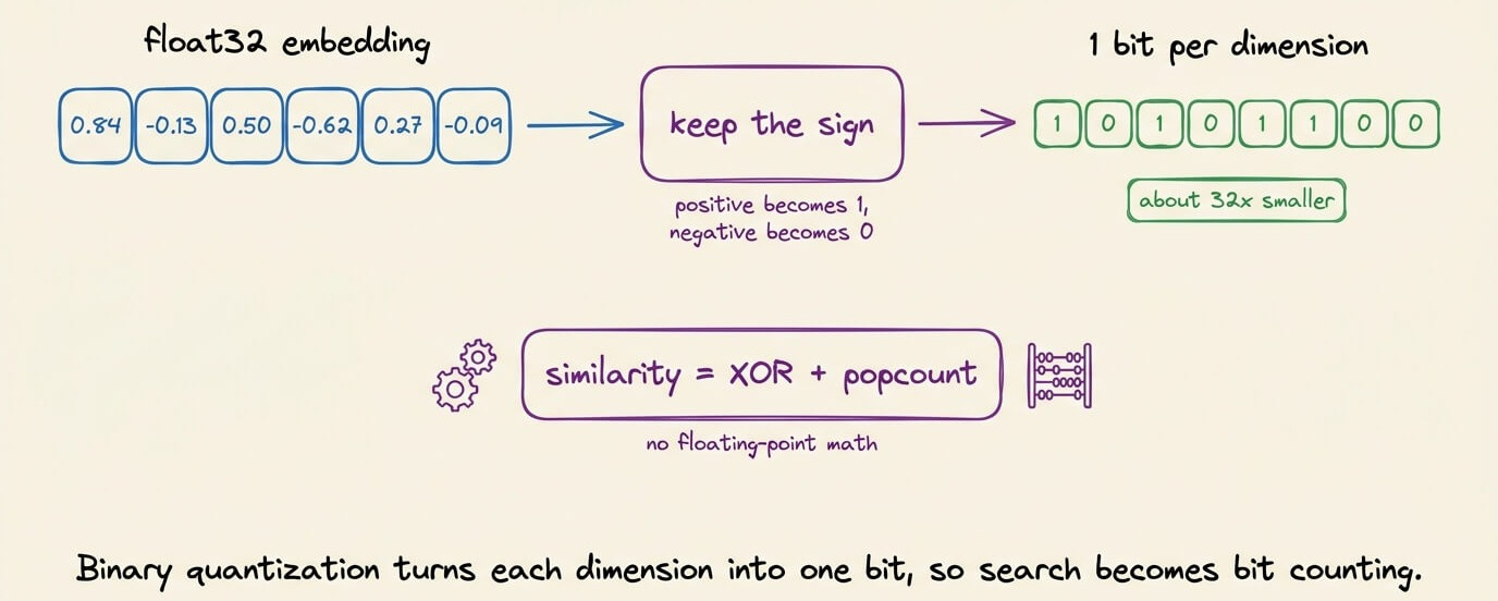
Similarity search can then use XOR and a population count instead of floating-point distance calculations.

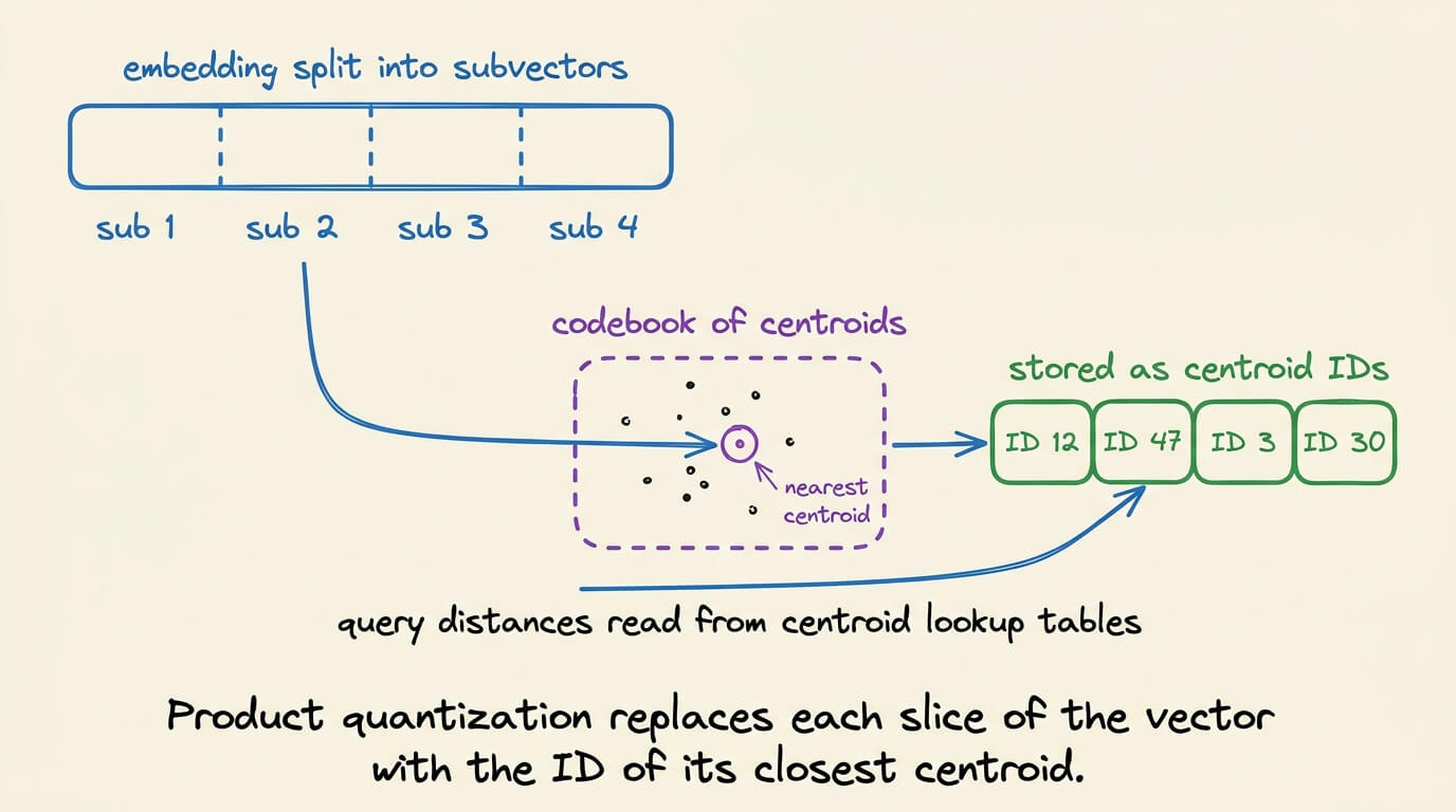
5) Product Quantization encodes subvectors as centroid IDs:

It splits a vector into subvectors and replaces each subvector with the ID of its nearest centroid.

Query distances are then approximated through centroid lookup tables.

In all of these setups, the compressed representation does not need to produce the final ranking.

Usually, you retrieve extra candidates from the compressed index, then recompute similarity using higher-precision document embeddings.

This is especially useful with binary quantization. One bit can preserve enough coarse structure but loses magnitude information.

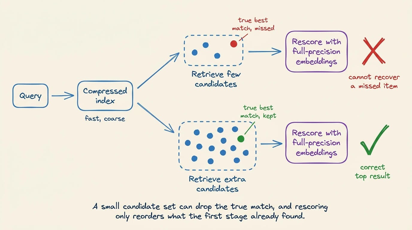
Rescoring improves the ordering, but it cannot recover an item missed by the initial compressed-retrieval stage.

Also, these methods can work together. An MRL embedding can be truncated first and quantized afterward, reducing both dimension and precision.

All of these techniques reduce the memory and compute a retriever uses once the index holds millions of vectors.

But it is a small part of building a retriever that works in production, which is what the RAG Systems course goes through. Here is the full series in order.

• Part 1 covers the foundations of a RAG system, including vector search, chunking, and embeddings →

• Part 2 shows how to evaluate a RAG system and which metrics tell you whether it actually works →

• Part 3 works on making retrieval faster and lighter on memory →

• Part 4 extends RAG to multimodal data like images and tables, not just text →

• Part 5 explains CLIP embeddings and multimodal prompting that put text and images in one space →

• Part 6 builds a full multimodal RAG system on real-world data →

• Part 7 brings in Graph RAG to use the relationships between entities during retrieval →

• Part 8 introduces late interaction with ColBERT for token-level matching between the query and the document →

• Part 9 builds vision-driven retrieval with ColPali that searches over document images directly →

• Part 10 walks through the first set of 16 practical techniques for production RAG →

• Part 11 continues with the remaining techniques from that set →

• Part 12 explains why RAG latency is really a prefill problem, the model reading the chunks rather than finding them →

• Part 13 starts the preloading arc by loading a corpus into cache before any query arrives →

• Part 14 compresses that cache and covers why most published methods still need a query first →

• Part 15 closes the preloading arc with the training-based methods and what running them in production takes →

Good day!