

Agents are repeating software’s dumbest mistake
The real moat in 2027 won’t be anything to do with the agent.
Instead, it’ll be about capturing full-stack trajectories.
Imagine two teams ship the same agent, on the same model, on the same day.
Your competitor ships it and moves on.
But you ship agents that learn from every session: where users stepped in, what they did by hand, what they keep asking for. Every week it picks up a few new skills, evals, and datasets.
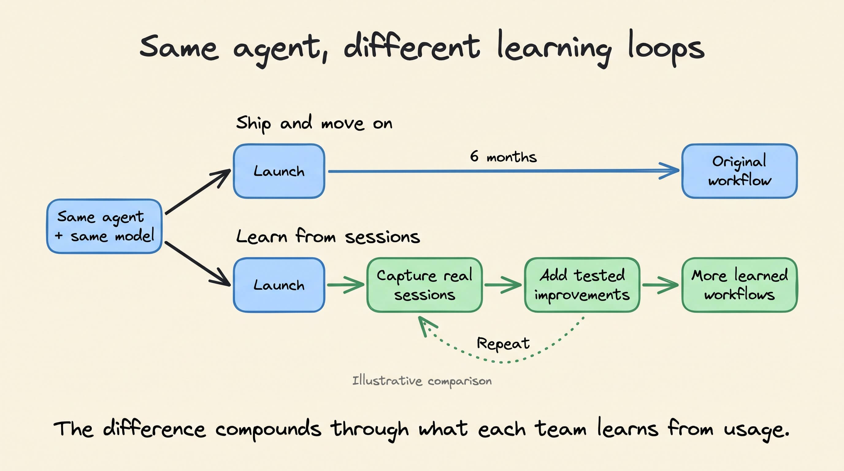
Six months later, you aren’t really competing on the same product anymore.
Because the advantage isn’t in the model but rather it’s in your users’ data.
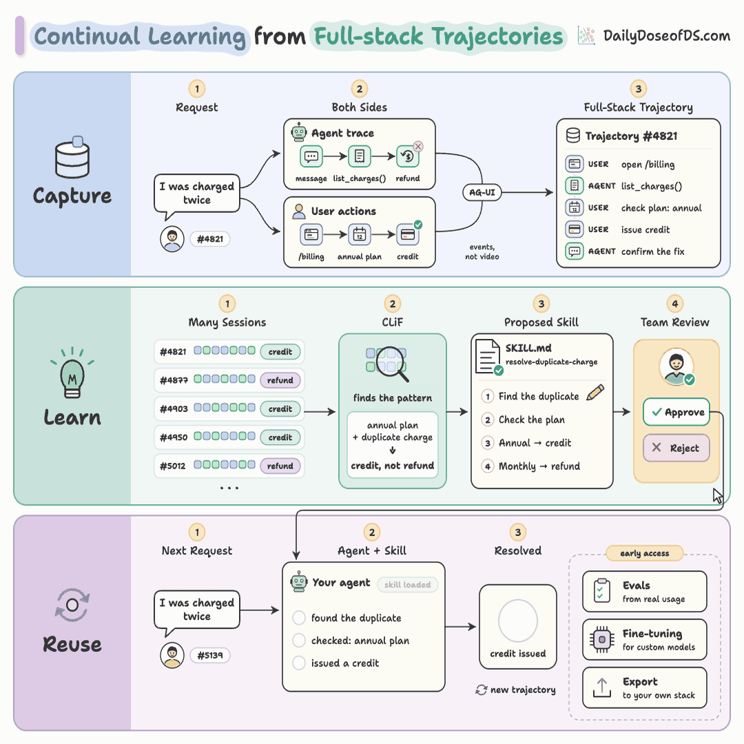
CLiF is a new learning platform built into CopilotKit that sees every trajectory:
The trace: every step the agent took
The product: everything the users did
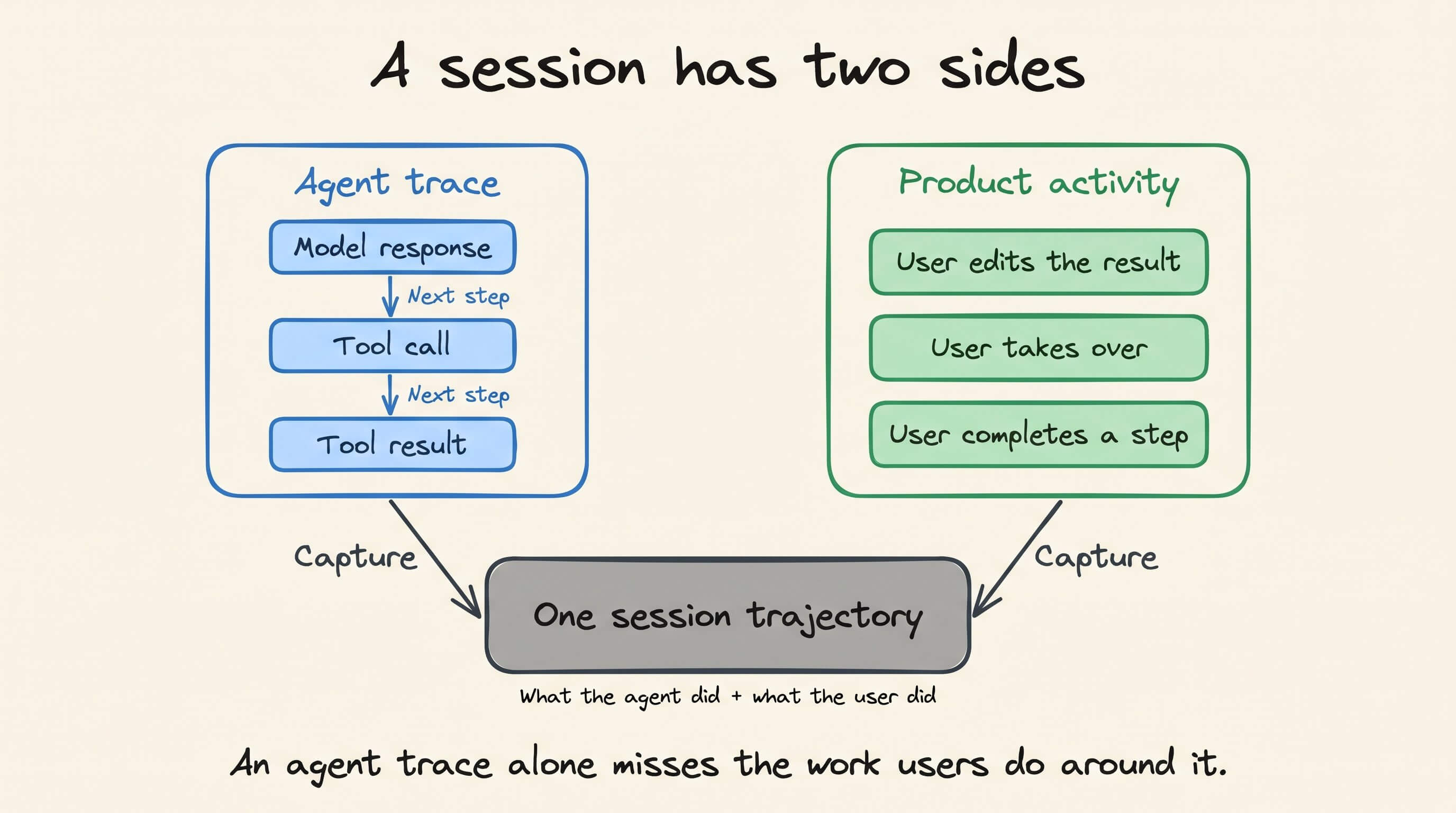
The AG-UI protocol already sits between the agent and the UI, so it sees both sides and then turns real sessions into exportable fullstack trajectories, evals, skills and fine-tuned models.
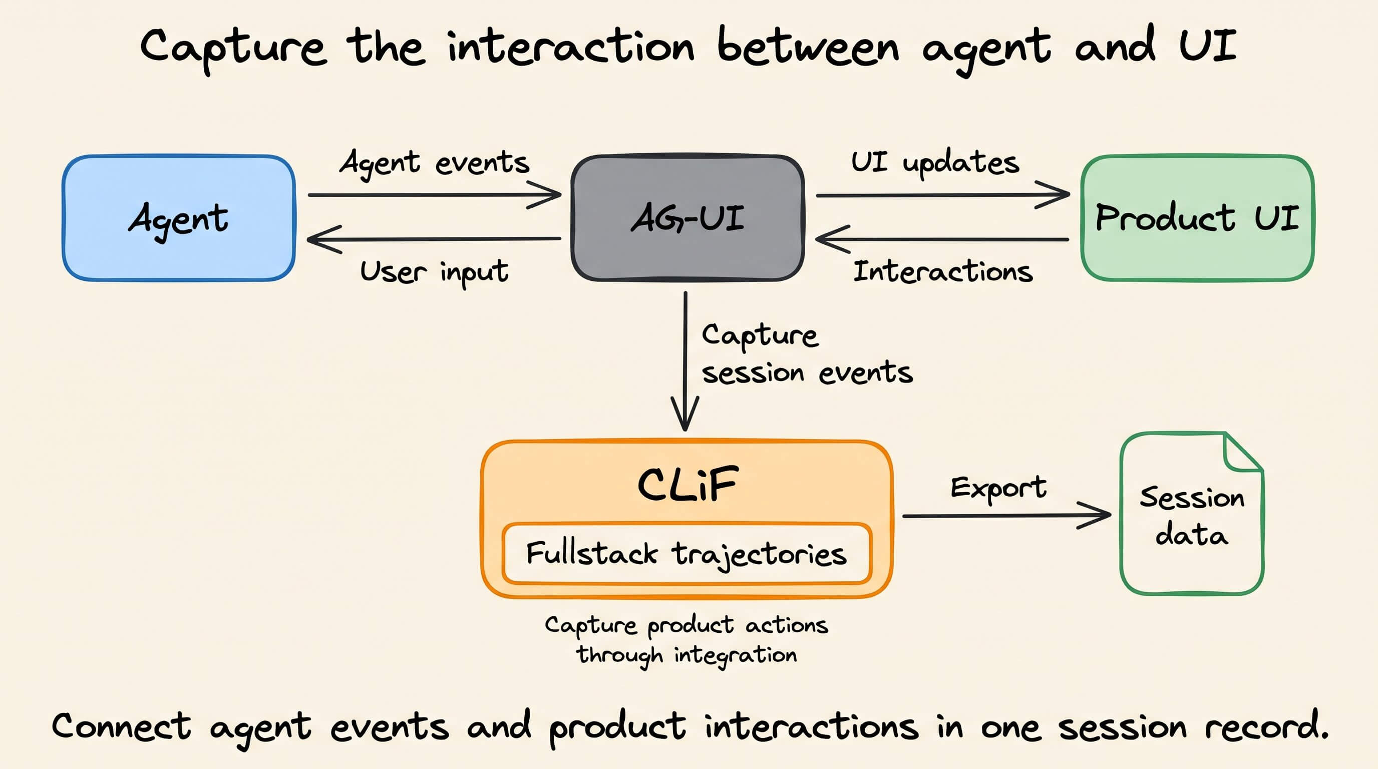
You can self-host it and access it here: http://go.copilotkit.ai/get-clif
Our suggestion if you’re building user-facing agents: start collecting this data now.
CLiF already implements the entire continual learning infrastructure you need to achieve that.
We are working on a hands-on demo of this and will share it soon. Stay tuned!
6 KV cache quantization approaches, explained visually:
Quantizing model weights doesn’t automatically shrink the KV cache.
Weights store the model’s learned parameters. The KV cache stores keys and values computed while processing a request. Reducing the precision of one doesn’t automatically change the other.
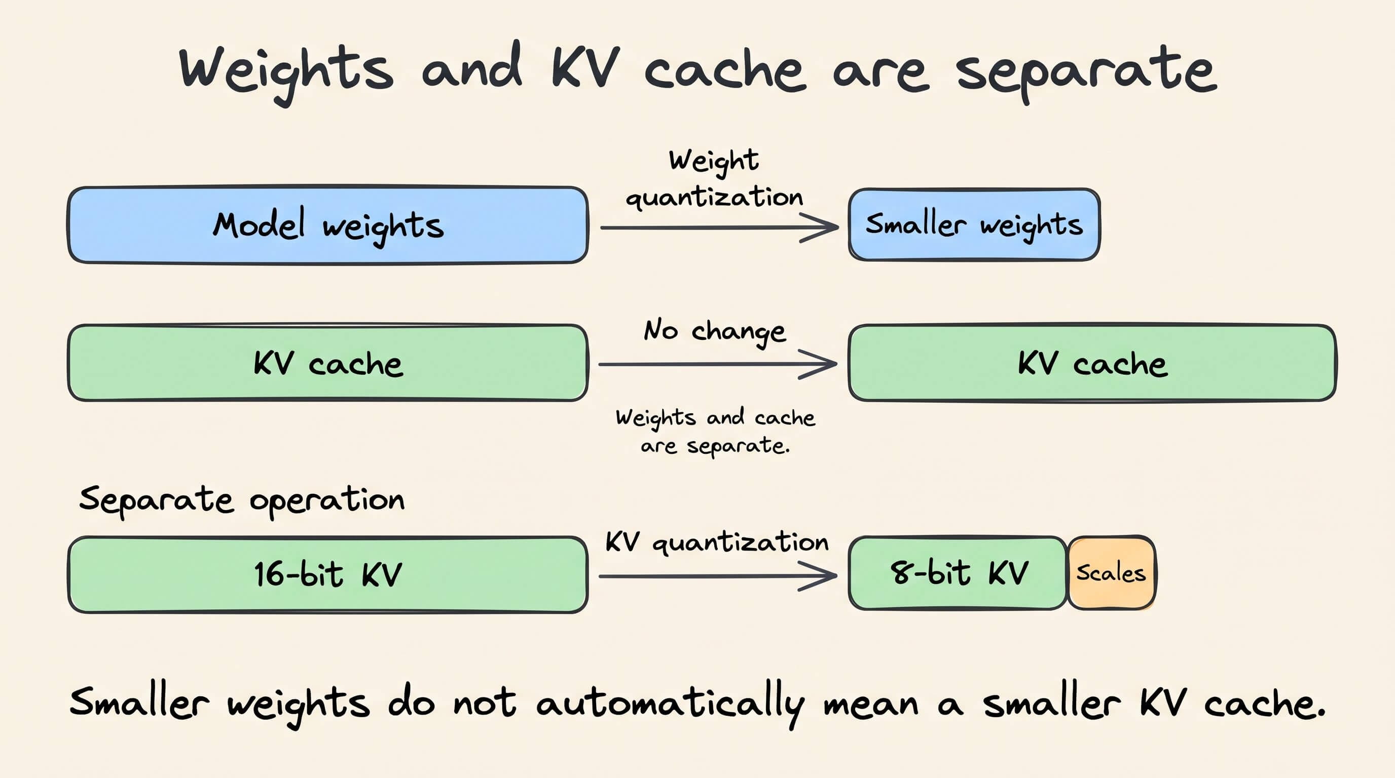
The cache grows as requests retain more tokens, and concurrent requests need room for their own entries. KV quantization reduces the bytes used to store those entries.
For instance, moving from 16-bit to 8-bit halves the raw KV data. The total saving is smaller once scales, other metadata, and any high-precision buffers are included.
The six approaches below describe different choices within KV quantization. Several can work together, such as 4-bit integers, small quantization groups, and a high-precision buffer for recent tokens.
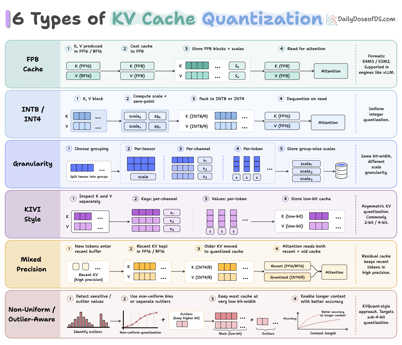
1. FP8 cache
A cache using FP16 or BF16 stores each number in 16 bits. FP8 stores it in 8 bits, so the same number of entries takes half the raw space.
A scaling factor adjusts the numbers to fit the FP8 range. The implementation retains the scale so the attention kernel can interpret the stored numbers correctly.
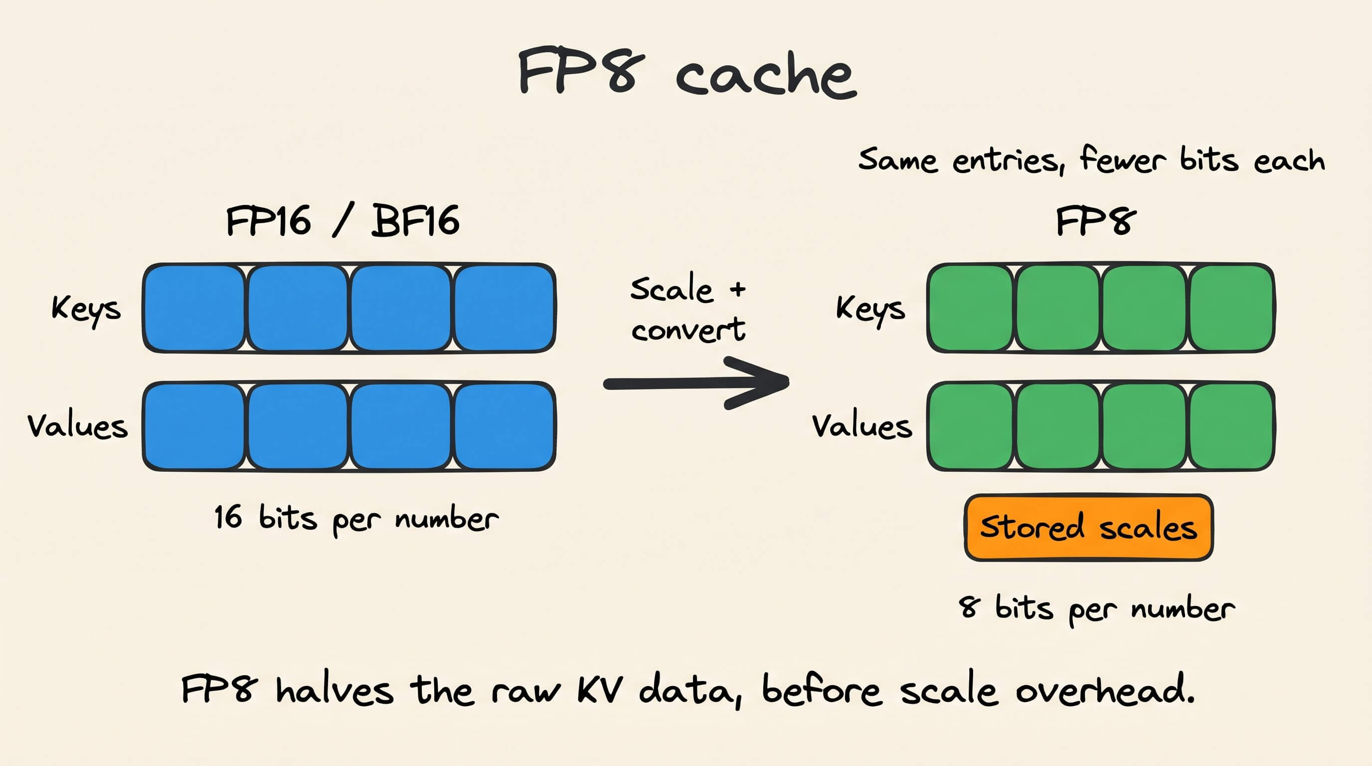
For example, 1 GiB of 16-bit KV data becomes 512 MiB of FP8 data, before scales and other overhead. The model weights occupy the same space unless they are quantized separately.
The serving engine and GPU need a compatible attention kernel. FP8 storage alone doesn’t establish how fast that kernel will run.
2. INT8 / INT4 cache
These methods represent cached numbers with 8-bit or 4-bit integers. A scale, and sometimes a zero-point, tells the kernel how those integers map back to approximate values.
INT8 has 256 possible integer levels. INT4 has 16, so it uses less storage but offers fewer choices when rounding a number.
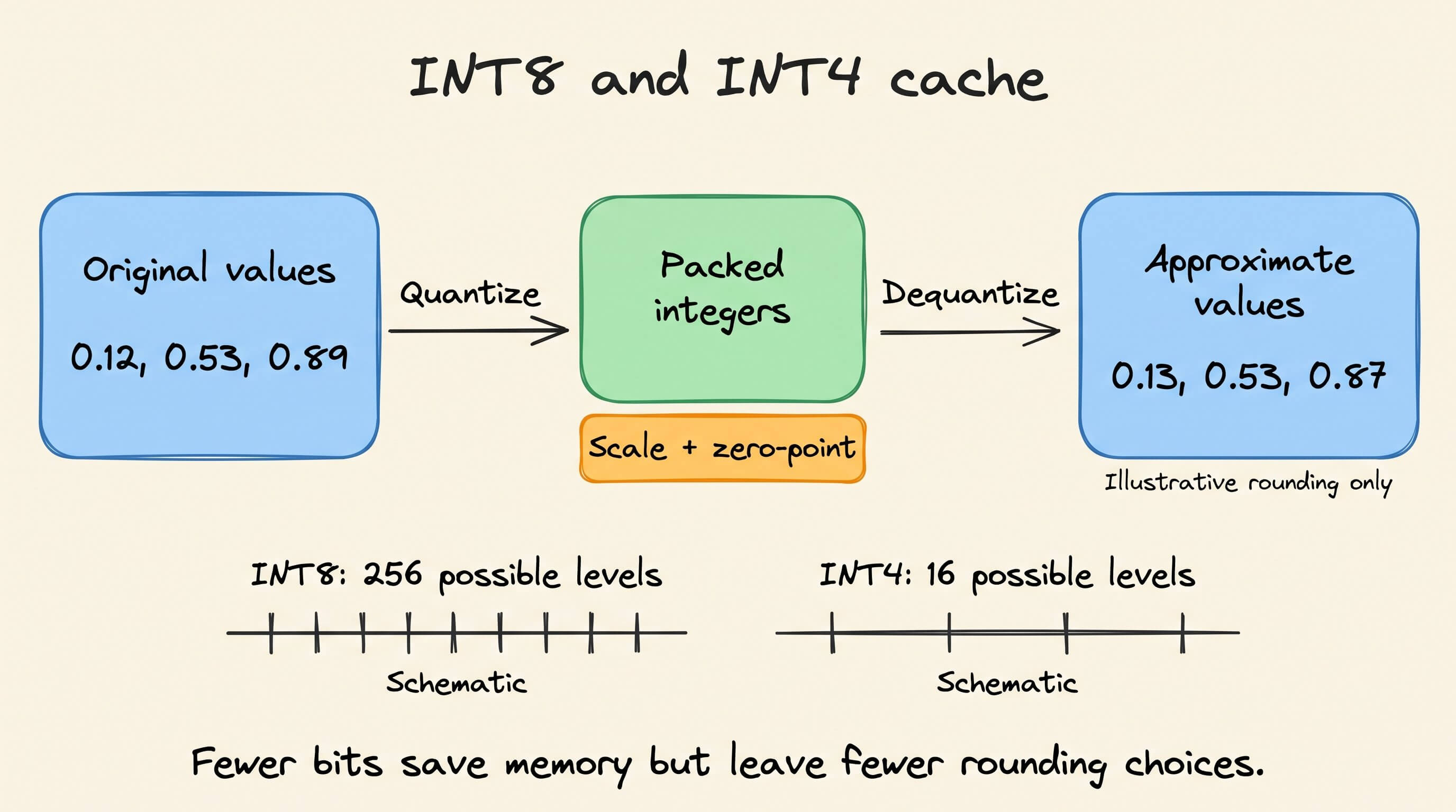
For example, two nearby values might round to the same level in INT4. After conversion back, attention can no longer distinguish them exactly.
The kernel unpacks and dequantizes the stored entries for attention, often within the attention computation itself. This work can offset some of the benefit of reading fewer bytes.
3. Quantization granularity
Granularity determines how many numbers share a scale. One scale can cover a whole tensor, or separate scales can cover channels, tokens, or smaller groups.
Suppose most numbers in a group lie between 0 and 1, but one is 20. A shared scale that includes 20 can leave fewer rounding levels available for distinguishing the smaller numbers.
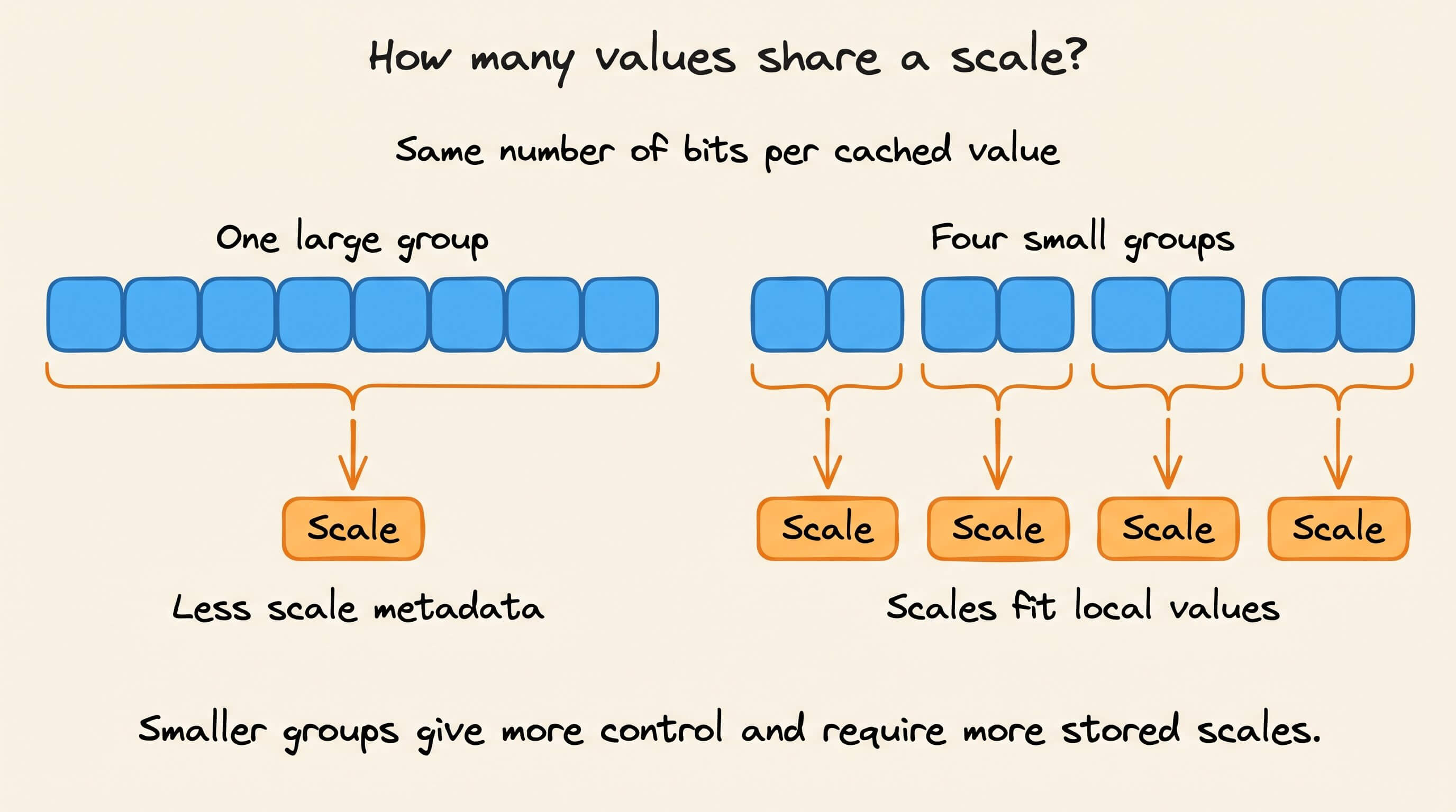
Smaller groups limit how many other numbers that outlier affects. But every group needs its own scale, which also occupies memory.
Two implementations can both use 4-bit values and still have different total memory use and accuracy because they share scales differently.
4. KIVI-style quantization
KIVI uses different grouping rules for keys and values. Its analysis found that unusually large key values tend to appear in particular channels, while values have a different pattern.
A channel is one coordinate of a key or value vector. KIVI groups keys from the same channel across a block of tokens, giving that channel its own scale within the block.
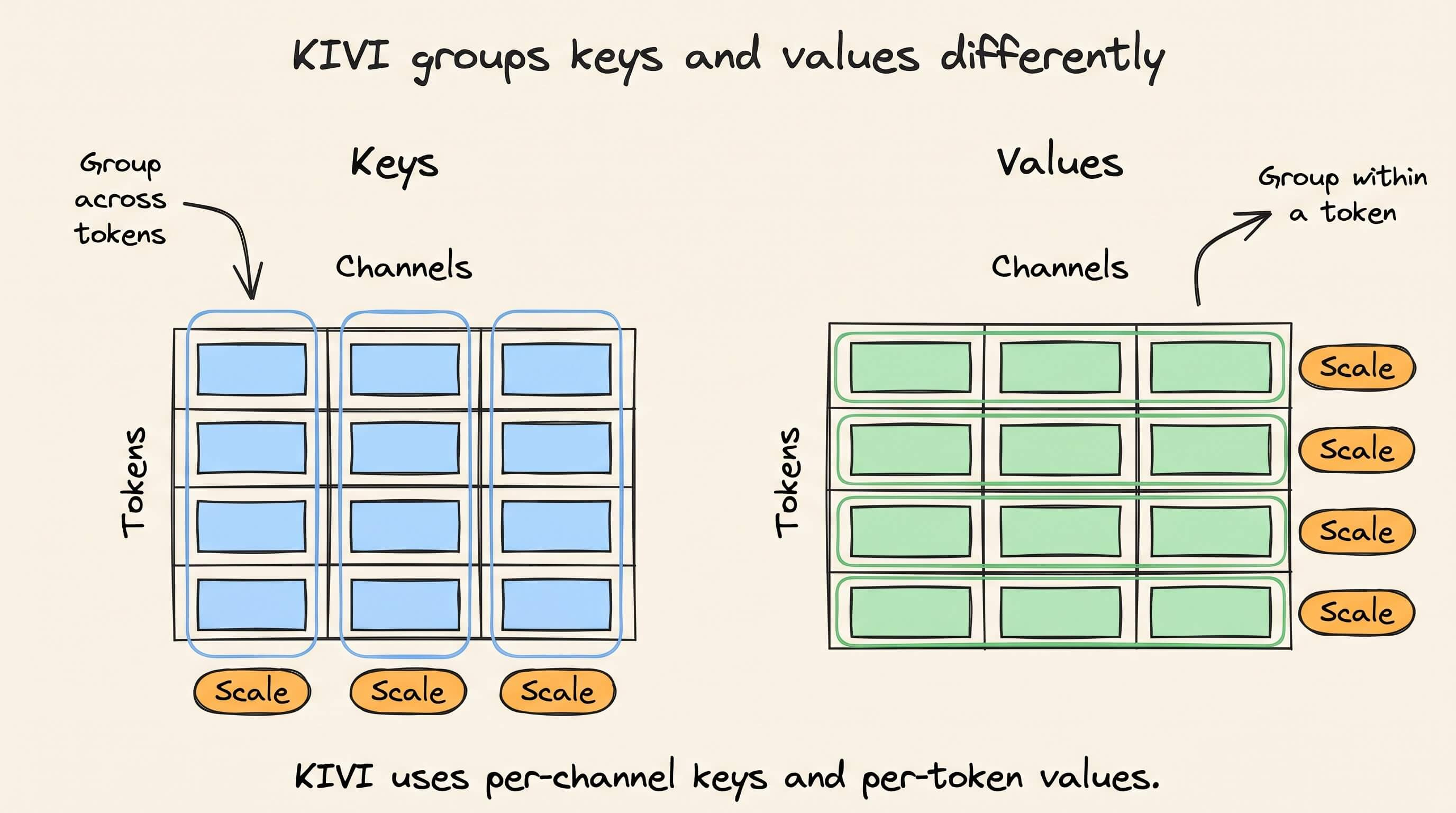
For values, it groups numbers within each token instead. A token’s value range therefore doesn’t set the scale for every other token.
The original method targets 2-bit KV storage without fine-tuning the model. Its grouping rules help control rounding error, but accuracy still needs checking on the model and workload being served.
5. Mixed precision
One mixed-precision approach keeps recent keys and values in a high-precision buffer while storing older entries in a quantized cache.
New entries enter the buffer first. As it fills, the implementation quantizes a block of entries and moves it into the compressed portion.
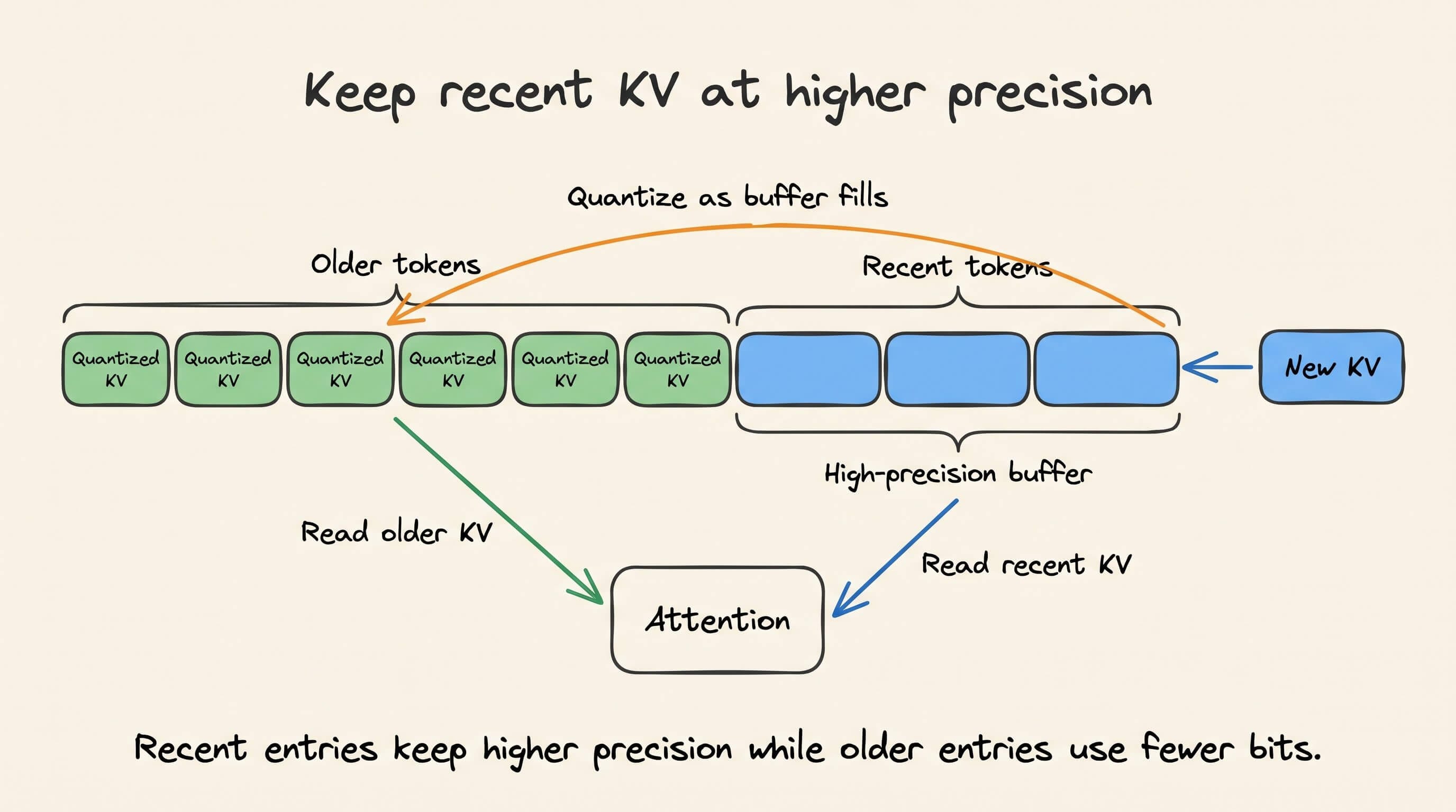
During decoding, attention reads both portions. Recent entries avoid quantization error while they remain in the buffer.
A larger buffer keeps more entries at higher precision, but reduces memory savings. This approach can also help collect enough tokens to quantize keys in blocks, as KIVI does.
6. Non-uniform / outlier-aware quantization
Uniform quantization rounds numbers to evenly spaced levels. Non-uniform quantization changes that spacing, assigning levels to better represent the value distribution or preserve sensitive values.
For example, if many numbers cluster near zero, more levels can be placed there rather than spread evenly across a wide range.
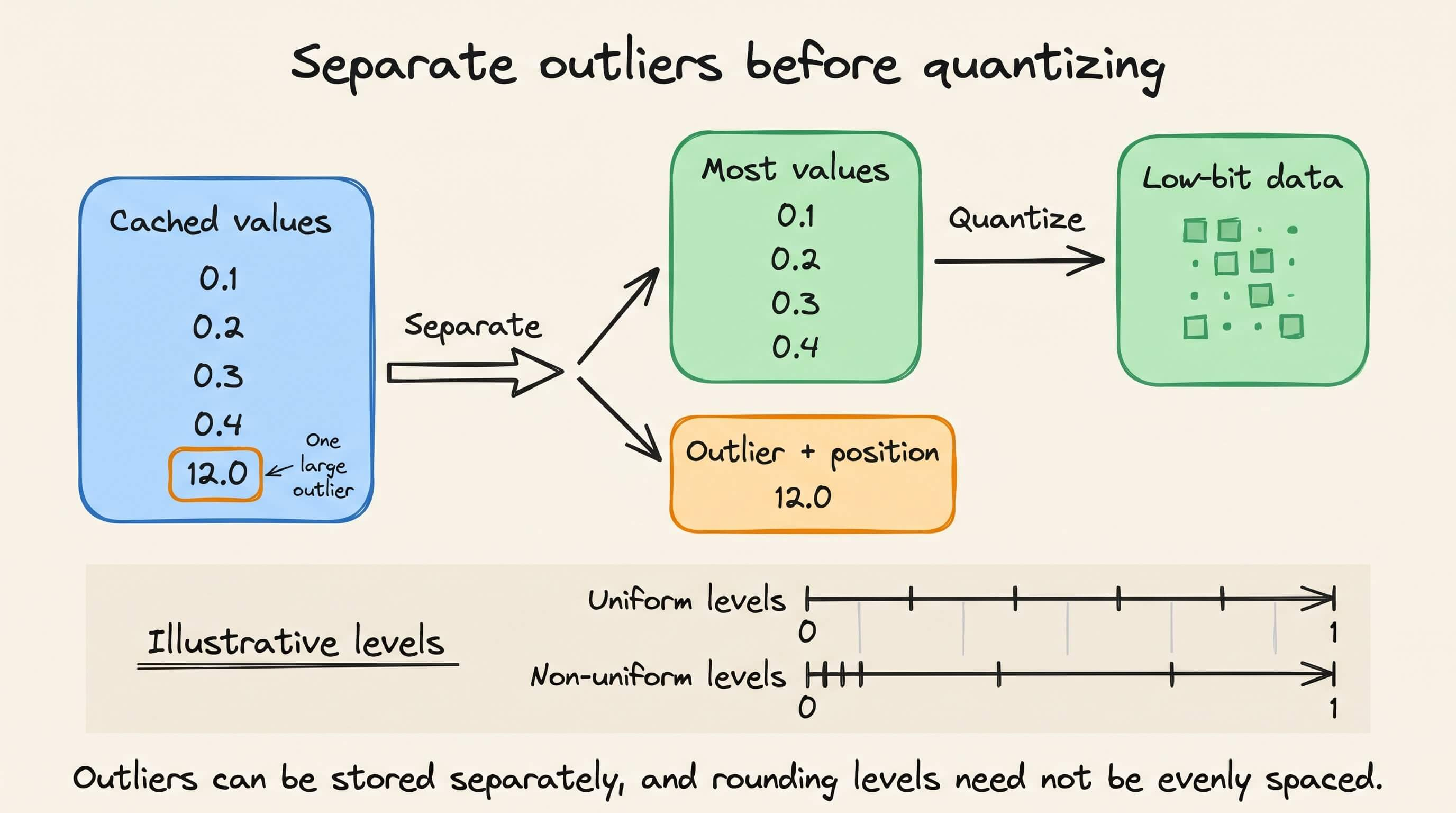
Outlier handling addresses a related problem. KVQuant separates unusually large values into sparse storage, keeping their positions so the kernel can account for them during attention.
The remaining values can then use a narrower range. The separate outliers and their positions add overhead, so the memory cost includes more than the low-bit data alone.
Check the saving against the cost
A smaller cache can fit longer contexts or more requests on the same GPU. Faster decoding depends on whether reduced memory traffic outweighs the extra quantization work.
Compare against an unquantized cache using the same model, prompts, output lengths, and concurrency. Check total memory use, decoding latency, and answer quality on the long-context tasks that matter for the application.
We have covered every bit of it in the LLMOps course, starting from fundamentals to production:
Read Part 2 on understanding the core building blocks of LLMs →
Read Part 3 on the key components of LLMs, focusing on the attention mechanism, architectures like transformers and mixture-of-experts, and the fundamentals of pretraining and fine-tuning →
Read Part 4 on decoding strategies, generation parameters, best practices, and the broader lifecycle of LLM-based applications →
Read Part 5 on context + prompt engineering from a system perspective, in-context learning, types of prompts, and different prompting techniques →
Read Part 6 on prompt versioning, defensive prompting, and techniques like verbalized sampling, role prompting, and more →
Read Part 7 on context engineering, covering context types, context construction principles, and retrieval-centric techniques for building high-signal inputs →
Read Part 8 on memory, dynamic, and temporal context in LLM systems, covering short and long-term memory, dynamic context injection, and common failure modes in agentic applications →
Read Part 9 on evaluation methods and approaches for LLM-based applications, primarily focusing on building a strong understanding of the fundamental concepts →
Read Part 10 on evaluation benchmarks in LLM applications, with task-specific methodologies, and the core tooling for evaluation of LLM apps →
Read Part 11 on evaluation of multi-turn systems, tool use evaluations, tracing, and red teaming →
Read Part 12 on LLM fine-tuning, parameter-efficient methods like LoRA and QLoRA, and alignment techniques such as RLHF, DPO, and GRPO →
Read Part 13 on LLM inference optimization, KV caching, PagedAttention, FlashAttention, speculative decoding, and model parallelism →
Read Part 14 on the fundamentals of LLM serving, including API-based access, inference with vLLM, and practical decisions.
And we also wrote an open-access KV Cache Engineering article covering quantization and other ways to reduce cache memory, with code examples and their trade-offs.
The evolution of the retrieval layer
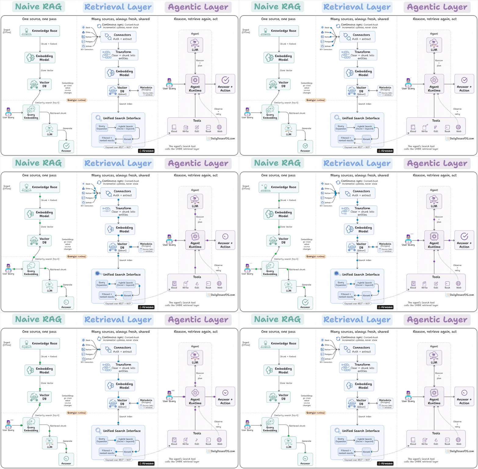
Google and Anthropic agree on one thing about RAG that retrieval is no longer a pipeline you build once.
Instead, it is a tool that something else calls.
Anthropic’s MCP exposes retrieval as a tool an agent can call.
Google now ships retrieval the same way, with its RAG Engine sitting under the Gemini agent platform alongside MCP servers.
That shift sounds small, but it changes the entire architecture underneath.
Today, let’s break down why classical RAG isn’t ideal in production, what a standing retrieval layer looks like, and how agents consume it.
Classical/Naive RAG
Naive RAG runs as a one-time pipeline inside a single app. A knowledge base gets chunked, embedded, and written to a vector DB.
At query time, the user’s query hits that vector DB for a similarity search, and the retrieved chunks go to the LLM.
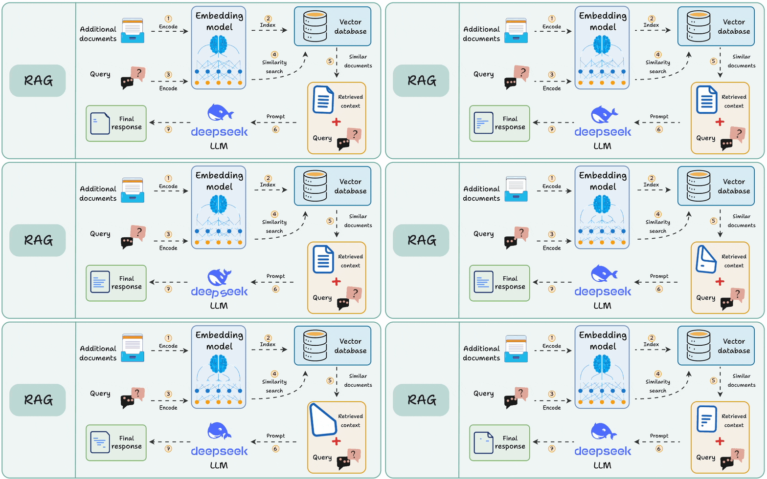
This works when the answer lives in one corpus that rarely changes. It breaks on two fronts that show up immediately at scale.
The first is staleness. The embeddings reflect the source at the moment of indexing. When a doc changes in Notion or a row updates in Postgres, the vectors still point at the old content until someone reruns the pipeline.
The second is duplication. The retrieval logic is welded to one application. A second app, or an agent, that needs the same data has to rebuild the same connectors, chunking, and embedding from scratch.
Retrieval as a standing layer
The fix is to stop treating retrieval as a step inside the app and start treating it as a standing layer underneath it. A retrieval layer separates ingestion from query, and runs ingestion continuously instead of once.
On the ingest side, connectors pull from many sources, handle auth and extraction, chunk into entities, embed, and write to a vector store with a metadata store alongside it for source links and versions.
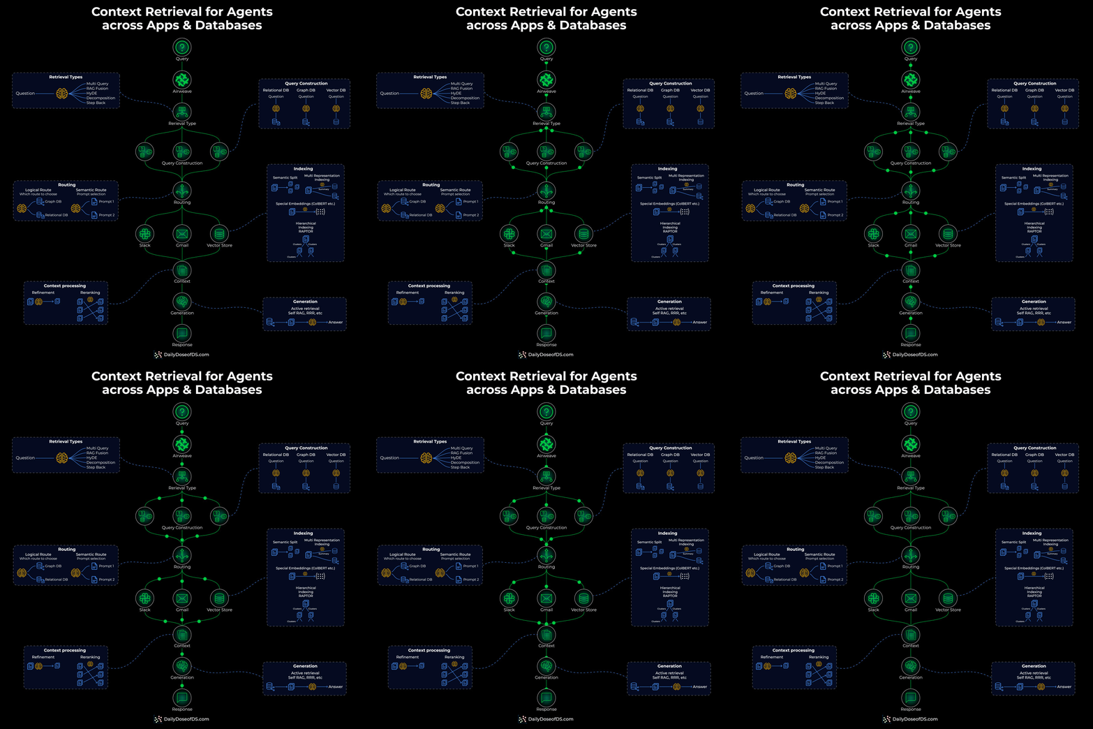
A sync process watches for changes and updates only what changed, using content hashing so unchanged data is not re-embedded.
On the query side, a request gets expanded, run through hybrid search that combines neural and keyword retrieval, then reranked before results come back with their source attribution.
The key property is that this layer is owned by no single app. It is exposed over an API, so a RAG chatbot and an autonomous agent can both query the same index.
How agents alter this scenario
An agent does not run retrieval once at the start.
It reasons, decides it needs context, calls search, reads the result, and decides whether to search again with a refined query. Retrieval becomes a tool inside a loop, not a fixed first step.
And the tool the agent calls is the retrieval layer.
The agent’s search function and the RAG app’s retrieval are the same query path into the same synced store.
They were never separate systems. Instead, one was just drawn inside the app, and the other was pulled out and shared.
👉 Over to you: Is moving retrieval out of the app and into a shared layer the right call for your stack?
Good day!