A Simple Technique to Robustify Linear Regression to Outliers

...And intuitively devising a new regression loss function.

The biggest problem with most regression models is that they are sensitive to outliers.

Consider linear regression, for instance.

Even a few outliers can significantly impact Linear Regression performance, as shown below:

Linear regression fit affected by outliers

And it isn’t hard to identify the cause of this problem.

Essentially, the loss function (MSE) scales quickly with the residual term (true-predicted).​

Mean Squared Error (MSE) loss function

Thus, even a few data points with a large residual can impact parameter estimation.

Huber loss (or Huber Regression) precisely addresses this problem.

In a gist, it attempts to reduce the error contribution of data points with large residuals.

How?

One simple, intuitive, and obvious way to do this is by applying a threshold (δ) on the residual term:

• If the residual is smaller than the threshold, use MSE (no change here).

• Otherwise, use a loss function which has a smaller output than MSE — linear, for instance.

This is depicted below:

Huber vs. MSE loss function

• For residuals smaller than the threshold (δ) → we use MSE.

• Otherwise, we use a linear loss function which has a smaller output than MSE.

Mathematically, Huber loss is defined as follows:

Huber regression loss function

Its effectiveness is evident from the image below:

Linear Regression vs. Huber Regressor

• Linear Regression is affected by outliers

• Huber Regression is more robust.

Now, I know what you are thinking.

How do we determine the threshold (δ)?

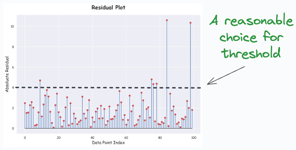
While trial and error is one way, I often like to create a residual plot. This is depicted below:

The below plot is generally called a lollipop plot because of its appearance.

Residual plot

• Train a linear regression model as you usually would.

• Compute the residuals (=true-predicted) on the training data.

• Plot the absolute residuals for every data point.

One good thing is that we can create this plot for any dimensional dataset. The objective is just to plot (true-predicted) values, which will always be 1D.

Next, you can subjectively decide a reasonable threshold value δ.

---

In fact, here’s another interesting idea.

By using a linear loss function in Huber regressor, we intended to reduce the large error contributions that would have happened otherwise by using MSE.

Thus, we can further reduce that error contribution by using, say, a square root loss function, as shown below:

MSE vs. Huber vs. DailyDoseofDS loss function

I am unsure if this has been proposed before, so I decided to call it the DailyDoseofDataScience Regressor 😉.

It is clear that the error contribution of the square root loss function is the lowest for all residuals above the threshold δ.

This makes intuitive sense as well.

---

👉 Here’s a question for you: It only makes sense to specify a threshold δ >= 1. Can you answer why?

👉 If you liked this post, don’t forget to leave a like ❤️. It helps more people discover this newsletter on Substack and tells me that you appreciate reading these daily insights. The button is located towards the bottom of this email.

Thanks for reading!

---

Latest full articles

If you’re not a full subscriber, here’s what you missed last month:

• Deploy, Version Control, and Manage ML Models Right From Your Jupyter Notebook with Modelbit

• Model Compression: A Critical Step Towards Efficient Machine Learning.

• Generalized Linear Models (GLMs): The Supercharged Linear Regression.

• Gaussian Mixture Models (GMMs): The Flexible Twin of KMeans.

• Bayesian Optimization for Hyperparameter Tuning.

• Formulating the PCA Algorithm From Scratch.

To receive all full articles and support the Daily Dose of Data Science, consider subscribing:

---

👉 Tell the world what makes this newsletter special for you by leaving a review here :)

👉 If you love reading this newsletter, feel free to share it with friends!