A Visual and Intuitive Guide to What Makes ReLU a Non-linear Activation Function

An intuitive guide to ReLU that you always wanted to read.

Nov 26, 2023

Of all possible activation functions, most people struggle to intuitively understand how ReLU adds non-linearity to a neural network.

The confusion is quite obvious because, with its seemingly linear shape, calling it a non-linear activation function isn’t that intuitive.

An obvious question is: “How does ReLU allow a neural network to capture non-linearity?”

If you have ever struggled with this, then today, let me provide an intuitive explanation as to why ReLU is considered a non-linear activation function.

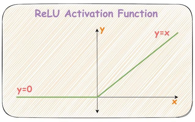
Let’s revisit the mathematical expression of the ReLU activation function and its plot.

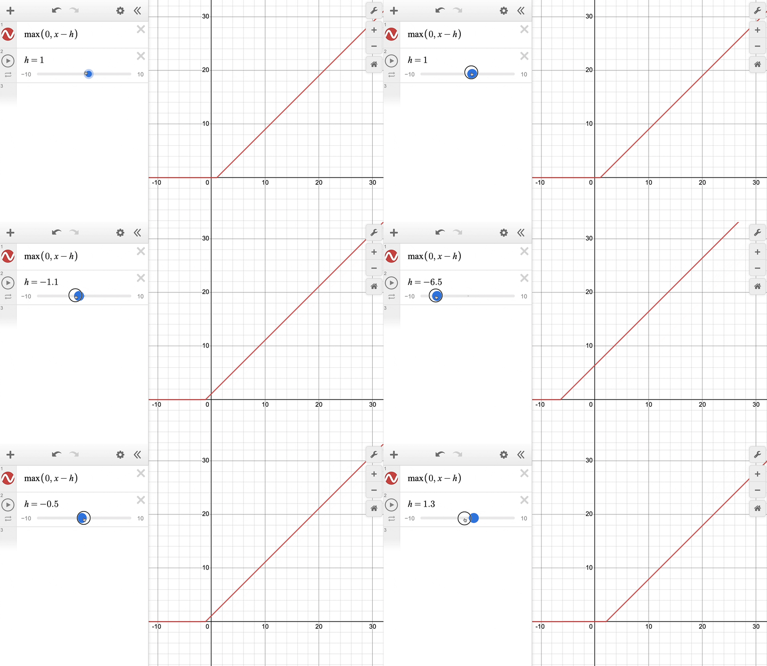
The above equation can be rewritten with a parameter h as follows:

Effectively, it’s the same ReLU function but shifted h units to the right:

Keep this in mind as we’ll return to it shortly.

Breaking down the output of a neural network

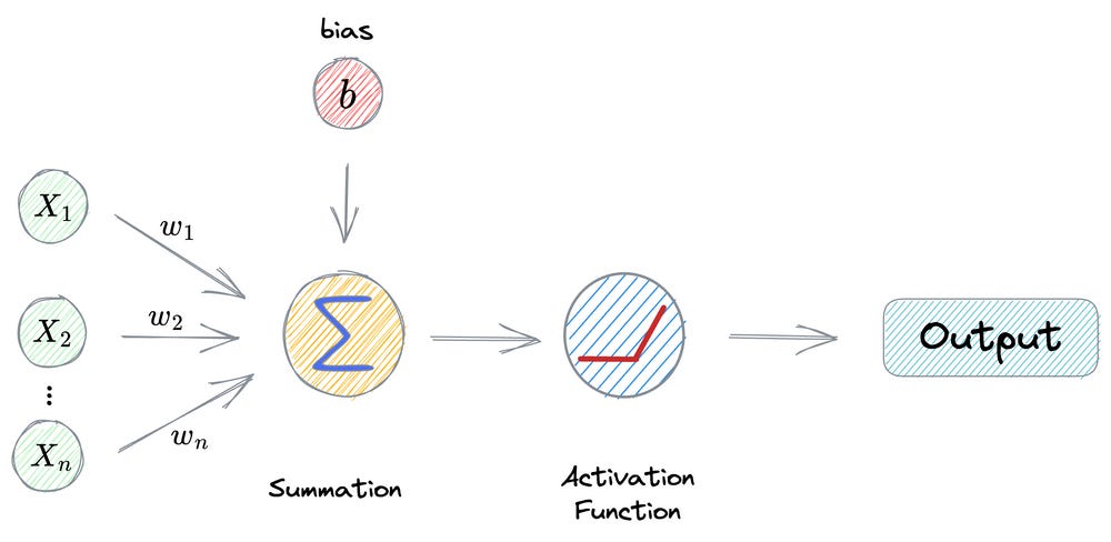
Consider the operations carried out in a neuron:

First, we have input from the previous layer (x₁, x₂, …, xₙ).
This is multiplied element-wise by the weights (w₁, w₂, …, wₙ).
Next, the bias term (b) is added, and every neuron has its own bias term.
The above output is passed through an activation function (ReLU in this case) to get the output activation of a neuron.

If we notice closely, this final output activation of a neuron is analogous to the ReLU(x−h) function we discussed earlier.

Now, let’s zoom out and consider all neurons in the last hidden layer.

The following image illustrates how neurons in this layer collectively contribute to the network’s output.

Essentially, the final output is a weighted sum of differently shifted ReLU activations computed in the last hidden layer.

Plotting dummy ReLU units

Now that we know what makes up the final output of a network, let’s plot the weighted sum of some dummy differently shited ReLU functions and see how the plot looks.

Let’s start with two terms:

In the above image, we notice that adding two ReLU terms changes the slope at a point.

Let’s add more ReLU terms to this.

This time, we see two bends in the final output function.

Let’s add more terms:

This time, we see even more bends in the final function of ReLU terms.

What does this tell us?

The above illustrations depict that we can potentially add more and more ReLU terms, each shifted and multiplied by some constant to get any shape of the curve, linear or non-linear.

The above equation has no restriction on the nature of the curve; it may be linear or non-linear.

The task is to find those specific weights (w₁, w₂, …, wₙ) which closely estimate the function f(x).

Theoretically, the precision of approximation can be entirely perfect if we add a ReLU term for each possible value of x.

X-squared demo

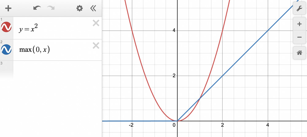
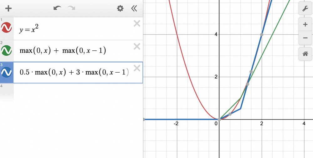
Let’s say we want to approximate y=x^2 for all x ∈ [0,2].

Thus, approximating with just one ReLU term → ReLU(x), we get:

Let’s see if adding another ReLU term helps → ReLU(x) + ReLU(x−1):

The green line is a better approximation than what we got with a single ReLU unit.

Let’s see if adjusting the weights helps.

The blue line looks even better than what we had earlier.

I hope you get where we are going.

The core point to understand here is that ReLU NEVER adds perfect non-linearity to a neural network.

Instead, it’s the piecewise linearity of ReLU that gives us a perception of a non-linear curve.

Also, as we saw above, the strength of ReLU lies not in itself but in an entire army of ReLUs embedded in the network.

This is why having a few ReLU units in a network may not yield satisfactory results.

This is also evident from the image below:

As shown above, as the number of ReLU units increases, the approximation also becomes better. At 100 ReLU units, the approximation appears entirely non-linear.

And this is precisely why ReLU is called a non-linear activation function.

Hope that was useful!

👉 If you liked this post, don’t forget to leave a like ❤️. It helps more people discover this newsletter on Substack and tells me that you appreciate reading these daily insights.