Activation Pruning for Model Compression (with implementation)

Removing 74% neurons with 0.5% accuracy drop.

Turn any data source into Agent-ready knowledge (open-source)

RAG can’t keep up with real-time data.

Airweave builds live, bi-temporal knowledge bases so that your Agents always reason on the freshest facts.

Supports fully agentic retrieval with semantic and keyword search, query expansion, and more across 30+ sources.

100% open-source.

GitHub repo → (don’t forget to star it)

We’ll share a hands-on demo on this tomorrow.

---

Activation pruning for model compression (with implementation)

A trained neural network always has neurons that do not substantially contribute to the performance.

But they still consume memory.

These can be removed without significantly compromising accuracy.

Let’s see how to identify them!

We covered 6 more model compression techniques here →

Also, the full MLOps crash course revolves around building production-grade and efficient ML systems with the right principles:

• ​Part 1 covered foundations and MLOps system principles →​

• Part 2 covered ML system lifecycle with hands-on project →​

• Part 3 covered reproducibility and versioning for ML systems →​

• ​Part 4 also covered reproducibility and versioning for ML systems →​

• Part 5 covered data and pipeline engineering →​

• Part 6 covered building scalable data pipelines →​

• Part 7 covered Spark, and orchestration + workflow management →​

• Part 8 covered the modeling phase of the MLOps lifecycle from a system perspective →​

• Part 9 covered fine-tuning and model compression/optimization →

Here are the steps:

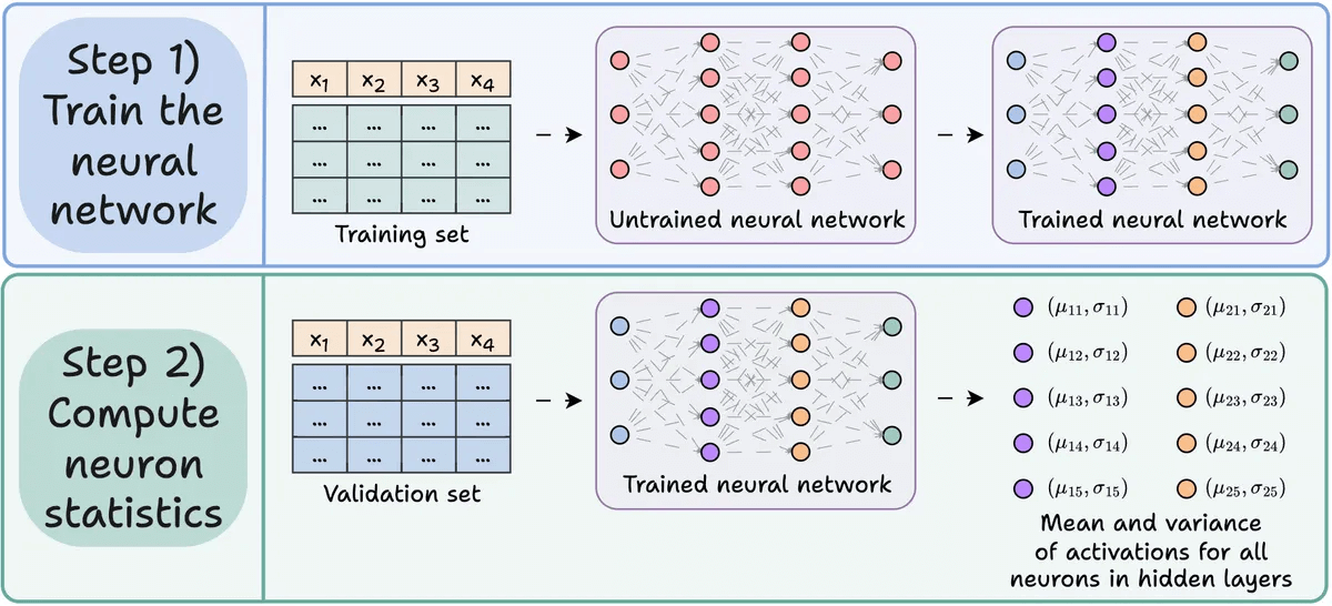
Step 1) Train the neural network as usual.

Step 2) Pass the validation set through the trained network, and for every neuron in the hidden layers, compute:

• The average activation

• The variance of activations (if activations can be -ve)

Step 3) Prune neurons that have a near-zero activation mean and variance since they have little impact on the model’s output.

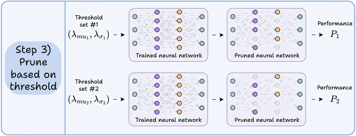
Ideally, plot the performance across several pruning thresholds to select the model that fits your size vs. accuracy tradeoffs.

Let’s look at the code.

We start by defining a simple neural network and train it.

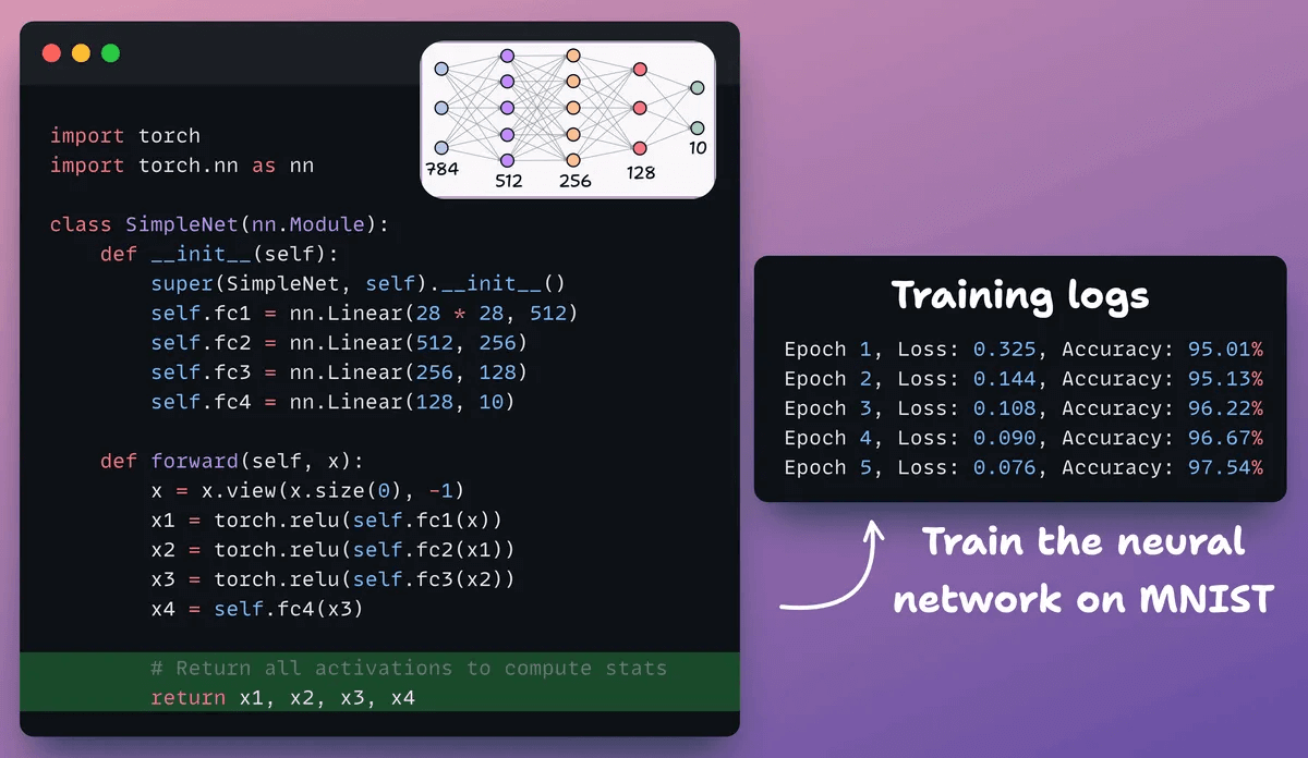
Since we shall compute neuron-level activations later for pruning, we return all the intermediate activations in the forward pass.

Next, we define two lists with three elements:

• One will store mean of activations

• Another will store std dev of activations

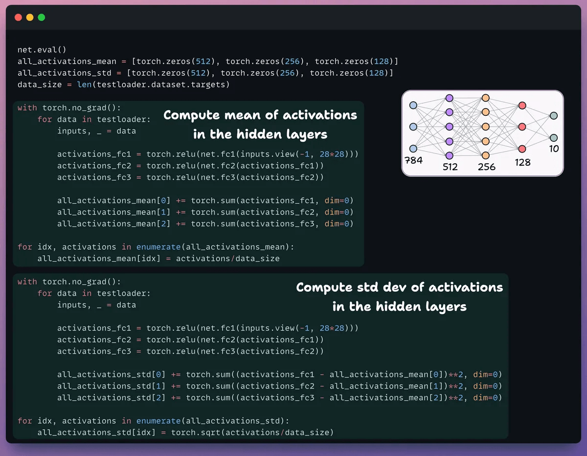
We pass the validation set through our model to compute these stats for each hidden layer.

At this point, let’s create a distribution plot of neuron-level statistics we generated above.

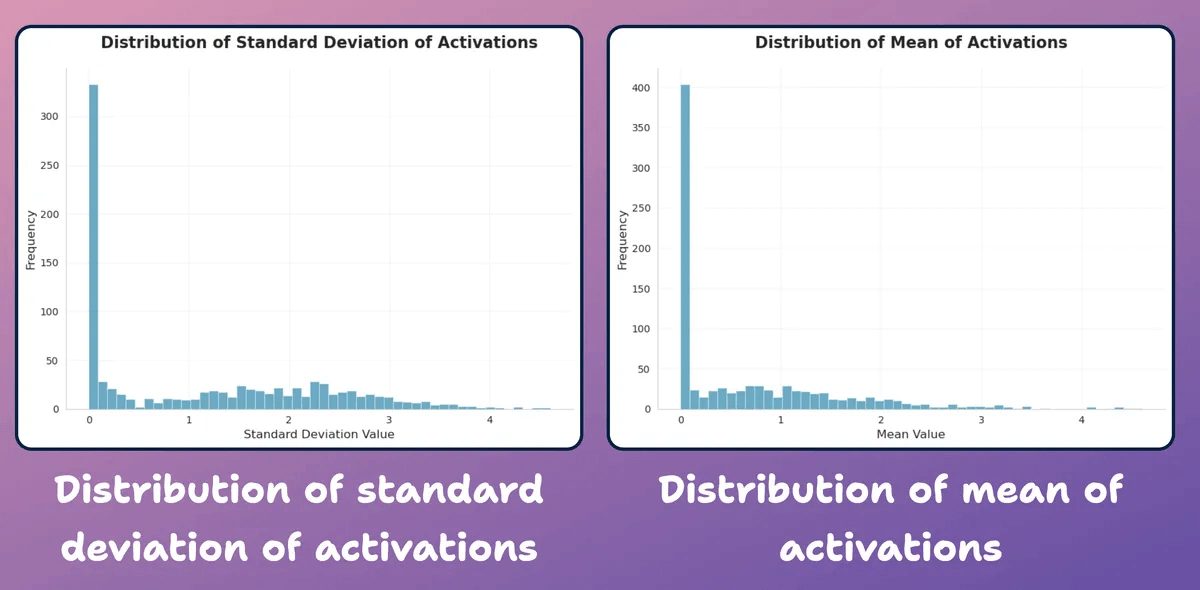
As depicted below, most neurons’ average activations and their std dev. are heavily distributed around near-zero values.

Let’s try to prune them next.

For pruning, we iterate over a list of thresholds and:

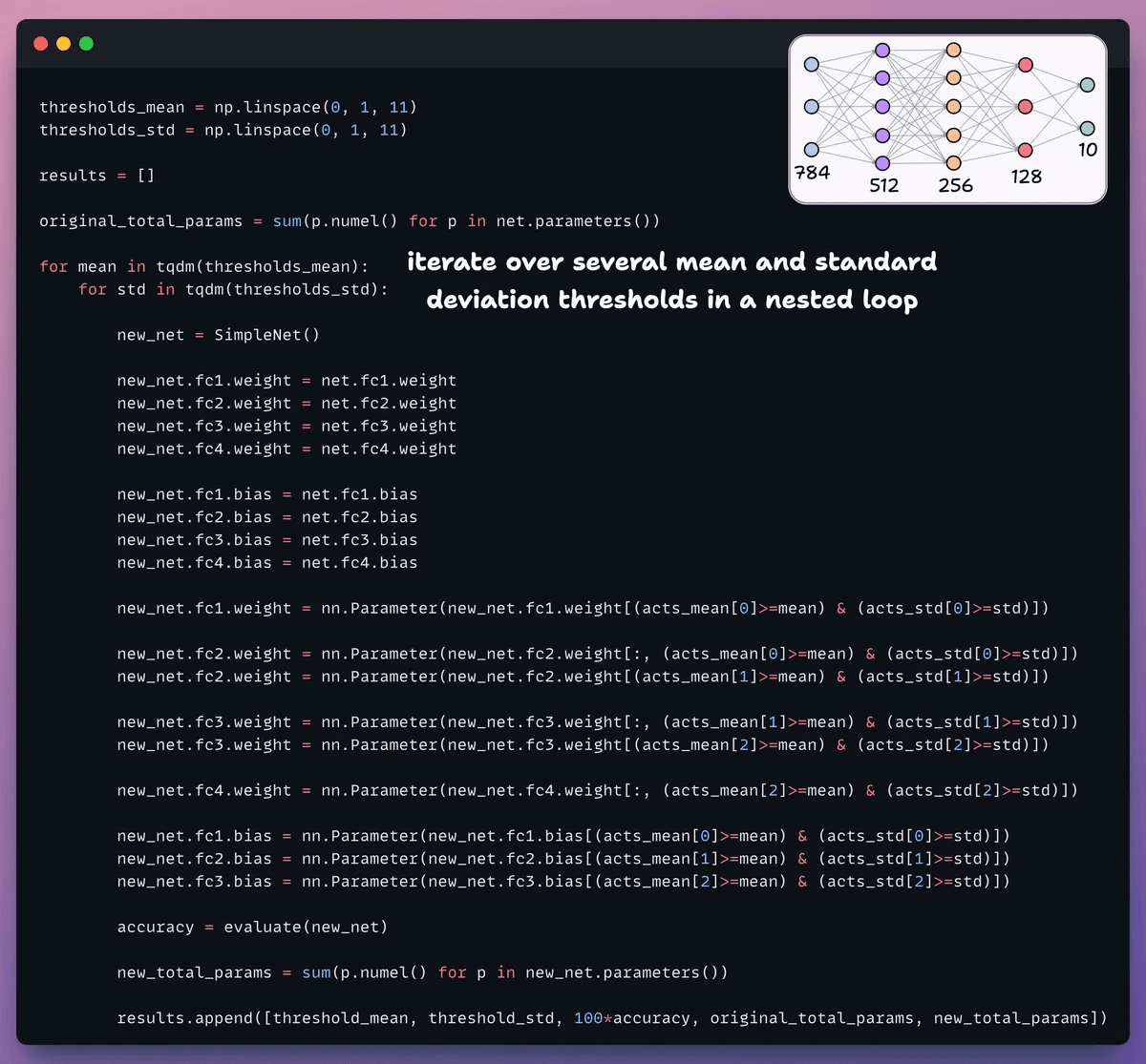
• Create a new network and transfer weights that pass the threshold.

• Evaluate the new network and calculate total params.

• Append the results to a list.

This table compares the pruned model’s accuracy and size reduction across several thresholds relative to the original model.

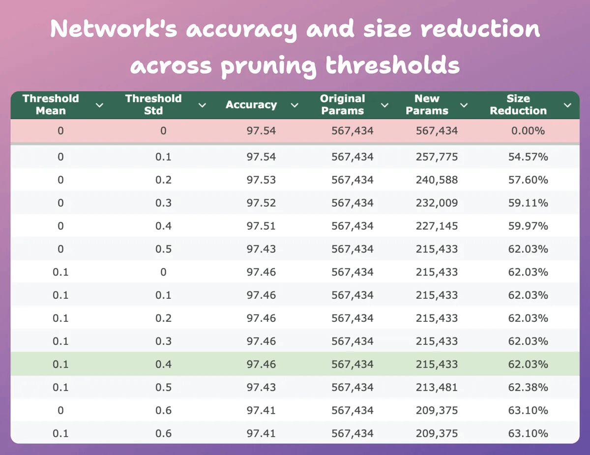
At mean=0.1 and std-dev=0.4:

• The model’s accuracy drops by 0.08%.

• The model’s size reduces by 62%.

That is a huge reduction.

Here’s another interesting result.

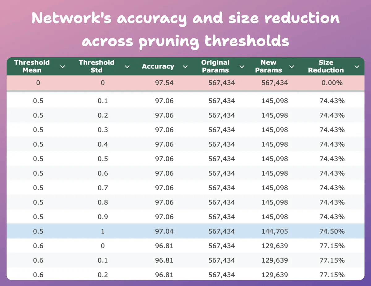
At mean=0.5 and std-dev=1:

• The model’s accuracy drops by 0.5%.

• The model’s size reduces by 74%.

So essentially, we get almost similar performance for 1/4th of the parameters.

Of course, there is a trade-off between accuracy and size. As we reduce the size, its accuracy drops (check the video).

But in most cases, accuracy is not the only metric we optimize.

Instead, several operational metrics like efficiency, memory, etc., are the key factors.

We covered 6 more model compression techniques here →

Also, the full MLOps crash course revolves around building production-grade and efficient ML systems with the right principles:

• ​Part 1 covered foundations and MLOps system principles →​

• Part 2 covered ML system lifecycle with hands-on project →​

• Part 3 covered reproducibility and versioning for ML systems →​

• ​Part 4 also covered reproducibility and versioning for ML systems →​

• Part 5 covered data and pipeline engineering →​

• Part 6 covered building scalable data pipelines →​

• Part 7 covered Spark, and orchestration + workflow management →​

• Part 8 covered the modeling phase of the MLOps lifecycle from a system perspective →​

• Part 9 covered fine-tuning and model compression/optimization →

Thanks for reading!