Condense Random Forest into a Decision Tree

Preserve generalization power while reducing run-time.

A couple of days back, I was reading my Bagging article to find some details.

While reading it, I thought of an interesting technique, using which, we can condense an entire random forest model into a single decision tree.

The benefits?

This technique can:

• Decrease the prediction run-time.

• Improve interpretability.

• Reduce the memory footprint.

• Simplify the model.

• Preserve the generalization power of the random forest model.

Let me explain what I thought.

---

Let’s fit a decision tree model on the following dummy dataset. It produces a decision region plot shown on the right.

It’s clear that there is high overfitting.

In fact, we must note that, by default, a decision tree can always 100% overfit any dataset (we will use this information shortly). This is because it is always allowed to grow until all samples have been classified correctly.

This overfitting problem is resolved by a random forest model, as depicted below:

This time, the decision region plot suggests that we don’t have a complex decision boundary. The test accuracy has also improved (69.5% to 74%).

This happens because of Bagging, and we discussed its mathematical motivation here: Bagging article.

Now, here’s an interesting thing we can do.

We know that the random forest model has learned some rules that generalize on unseen data.

So, how about we train a decision tree on the predictions generated by the random forest model on the training set?

More specifically, given a dataset (X, y):

• Train a random forest model. This will learn some rules from the training set which are expected to generalize on unseen data (due to Bagging).

• Generate predictions on X, which produces the output y'. These predictions will capture the essence of the rules learned by the random forest model.

• Finally, train a decision tree model on (X, y'). Here, we want to intentionally overfit this mapping as this mapping from (X) to (y') is a proxy for the rules learned by the random forest model.

This idea is implemented below:

The decision region plot we get with the new decision tree is pretty similar to what we saw with the random forest earlier:

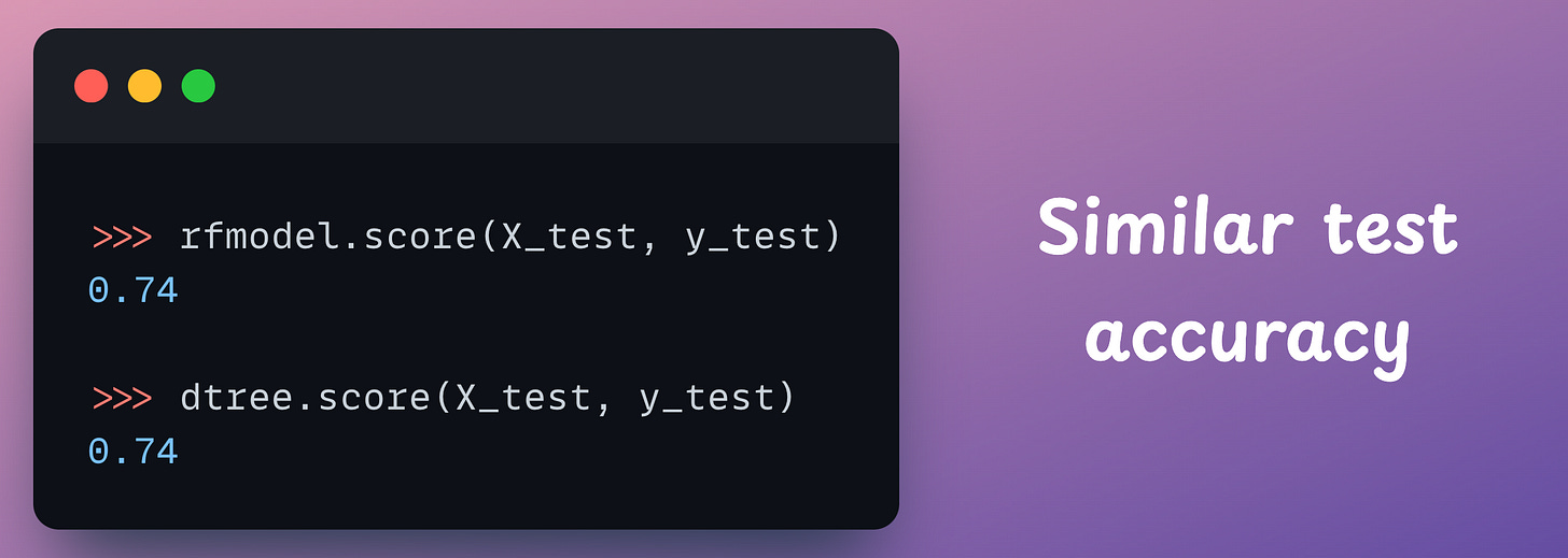
Measuring the test accuracy of the decision tree and random forest model, we notice them to be similar too:

In fact, this approach also significantly reduces the run-time, as depicted below:

Isn’t that cool?

Another rationale for considering doing this is that it adds interpretability.

This is because if we have 100 trees in a random forest, there’s no way we can interpret them.

However, if we have condensed it to a decision tree, now we can inspect it.

---

A departing note

As mentioned earlier, I have thought about this very recently. I tested this approach on a couple of datasets, and they produced promising results.

But it won’t be fair to make any conclusions based on just two instances.

While the idea makes intuitive sense, I understand there could be some potential flaws that are not evident right now.

So, I not saying that you should adopt this technique right away.

Instead, today’s newsletter is an appeal to test this approach on your random forest use cases and get back to me with what you discovered.

I will do a follow-up issue soon on this topic once I hear from some of you and I will share the observations.

In the meantime, I would also love to know your thoughts about this technique.

The code for this newsletter issue is available here: Random Forest to Decision Tree.

Thanks for reading!

---

Are you preparing for ML/DS interviews or want to upskill at your current job?

Every week, I publish in-depth ML deep dives. The topics align with the practical skills that typical ML/DS roles demand.

Join below to unlock all full articles:

Here are some of the top articles:

• [FREE] A Beginner-friendly and Comprehensive Deep Dive on Vector Databases.

• A Beginner-Friendly Guide to Multi-GPU Model Training.

• 11 Powerful Techniques To Supercharge Your ML Models.

• A Detailed and Beginner-Friendly Introduction to PyTorch Lightning: The Supercharged PyTorch

• Implementing LoRA From Scratch for Fine-tuning LLMs.

• Don’t Stop at Pandas and Sklearn! Get Started with Spark DataFrames and Big Data ML using PySpark.

• Federated Learning: A Critical Step Towards Privacy-Preserving Machine Learning.

• Sklearn Models are Not Deployment Friendly! Supercharge Them With Tensor Computations.

• Deploy, Version Control, and Manage ML Models Right From Your Jupyter Notebook with Modelbit

Join below to unlock all full articles:

---

👉 If you love reading this newsletter, share it with friends!

👉 Tell the world what makes this newsletter special for you by leaving a review here :)