Continuous Batching in LLMs

The technique behind vLLM's 23x throughput jump and the default scheduler in every serving engine.

Karpathy’s agentic engineering lifecycle, clearly explained:

The tooling to build agents is quite mature, so most of the work in shipping an agent isn’t writing the agent anymore.

It’s everything after, including scaffolding it, deploying it to a runtime, locking down its identity and network, evaluating it, and publishing it somewhere people can use.

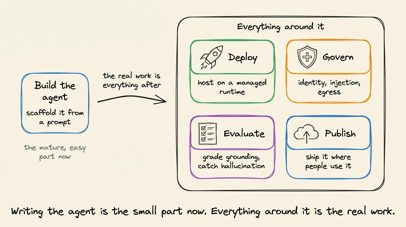
Each of those has traditionally lived in its own console, its own config, its own separate tool.

Google’s Agents CLI + skills implements procedures to condense the entire lifecycle into the coding agent itself, by prompting in plain English.

A setup command injects the lifecycle skills, so a single coding agent can carry an idea from an empty folder to a governed, published enterprise asset.

We mapped the full lifecycle in the diagram below. Here’s what each stage does.

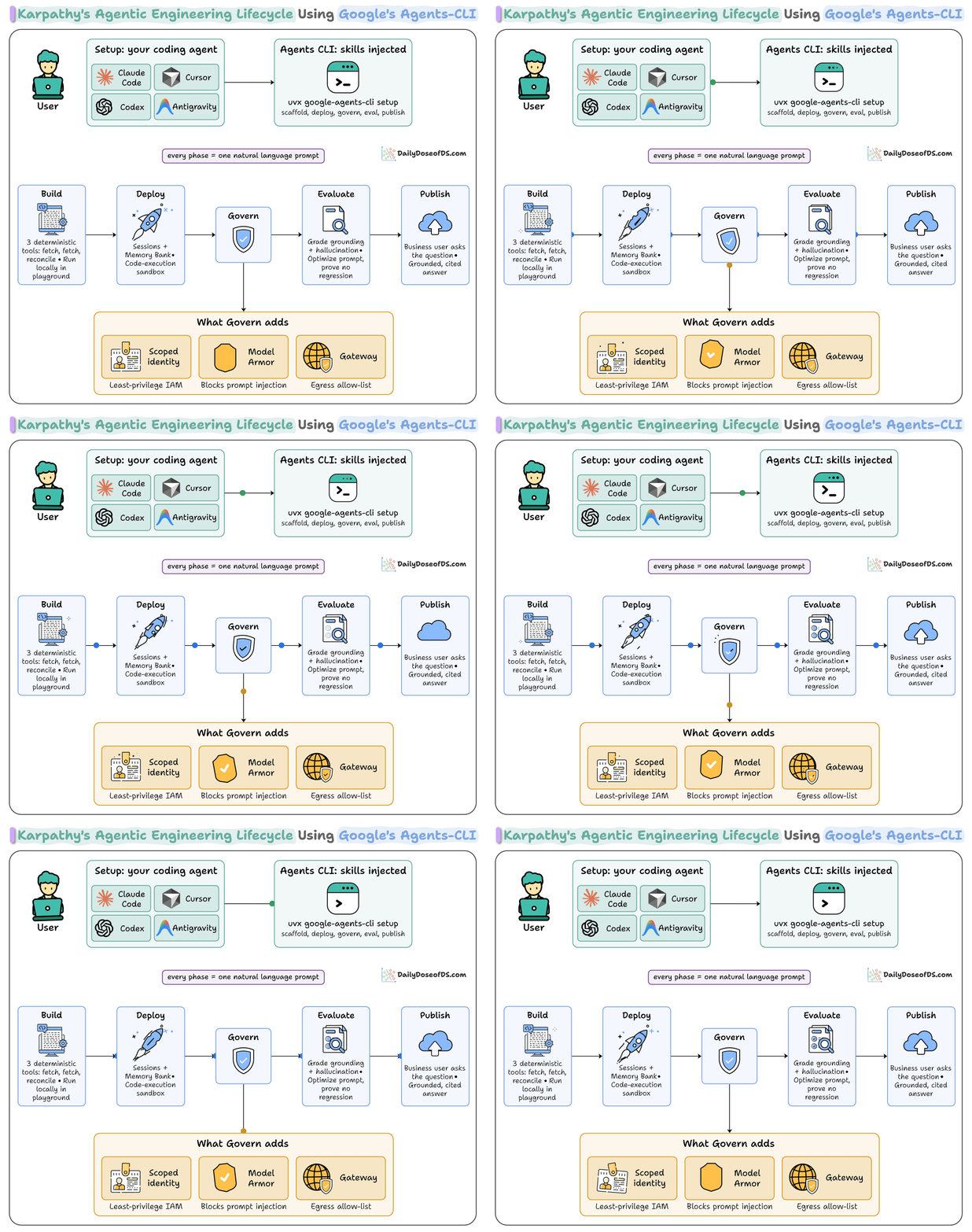
> Setup installs the skills into any coding agent (Claude Code, Cursor, Codex, Antigravity) from one command.

> Build scaffolds the agent and its deterministic tools from a prompt, then you run it locally in the playground.

> Deploy pushes it onto Agent Runtime with Sessions and Memory Bank, so it holds state across runs.

> Govern is the security stage, and Agents CLI drives all of it from prompts. It provisions a dedicated least-privilege identity, screens untrusted text for prompt injection through Model Armor, and confines the agent to an egress allow-list of hosts you approve.

> Evaluate checks grounding and hallucination, and then optimizes the prompt while proving no regression.

> Publish registers the agent into Gemini Enterprise for the whole org to use.

Every stage requires just natural-language prompts.

Agents CLI GitHub repo → https://github.com/google/agents-cli

(don’t forget to star it ⭐)

Thanks to Google Cloud for partnering with us today!

---

Continuous batching in LLMs

In traditional ML inference, a batch is usually represented as a matrix.

If there are inputs of varying lengths, then each input is padded or truncated to the same length, stacked into one tensor, and processed through a single forward pass to generate one prediction per row.

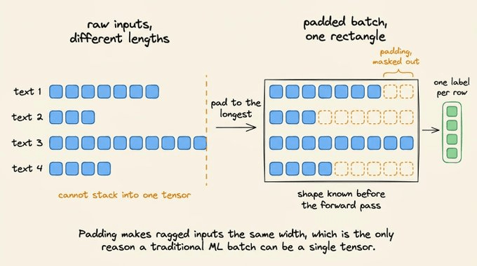
Every row costs the same, every row finishes at the same moment, and the full shape of the work is known before the pass starts. Batching there is a tensor-packing problem.

LLM decoding does not work on those principles.

Under the hood, one forward pass produces one token per sequence, so a request needs as many passes as it has output tokens, and nobody knows that count beforehand until the model emits a stop token.

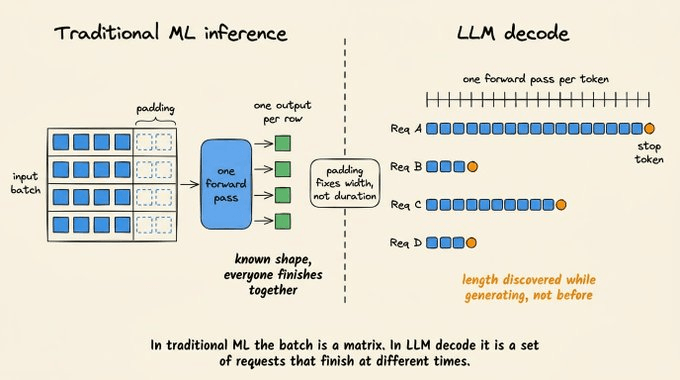
Padding can’t fix it, because the mismatch isn’t in the input width but rather in how long each request occupies the GPU.

So a batch fixed at the start runs at the pace of its slowest member.

Continuous batching is an approach implemented in most serving engines to avoid this problem. vLLM, SGLang, TGI, and TensorRT-LLM...all run it by default.

The core idea is to decide batch membership at every forward pass instead of once when the batch starts. A finished request leaves at the next pass and a waiting request takes its slot right there, so no slot sits reserved for work that’s already done.

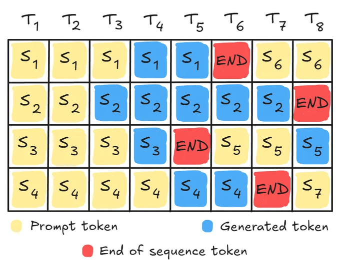
The scheduler underneath continuous batching is at the core of handling this process end-to-end, i.e., the loop that decides at every forward pass which requests get tokens and how many.

So let’s build it up from the problem, walk one scheduling step in order, and look at the measured gains once the mechanism is clear.

To dive deeper into the full LLMOps lifecycle, we have covered every bit of this in the LLMOps course, starting from fundamentals to production.

Start here →

---

Scheduler in traditional ML inference

A classifier takes a fixed-width input and returns a label.

Sequence models pad to a maximum length and mask the padding. Either way, the tensor going in has a known shape and the tensor coming out has a matching row count.

The reason to batch at all is that loading model weights out of HBM is a fixed cost per forward pass.

So if you stack 64 rows/inputs into a single pass and all those 64 rows share one weight read, the throughput rises:

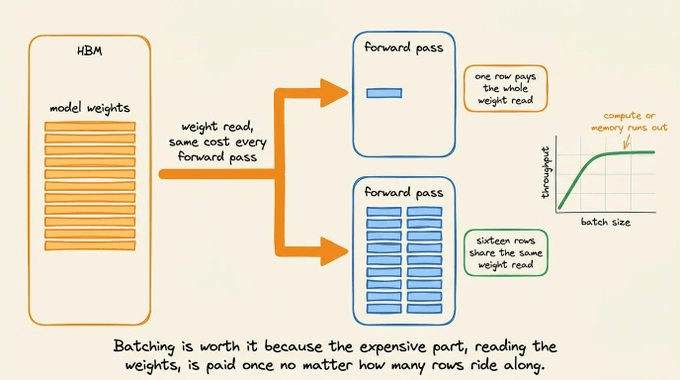
Serving that in practice is straightforward since you can simply fill a batch, run it, return every result, and start the next one.

No request carries state into the following pass, and no request outlives the batch it arrived in.

Nature of LLM inference

The decoding process in LLMs breaks three assumptions discussed above:

• Each pass generates a single token per sequence.

• The KV cache carries state forward into the next pass

• The number of passes a request needs is only known when it produces a stop token.

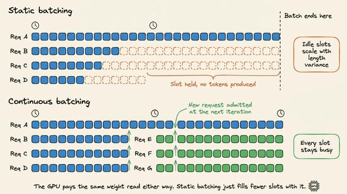
So a request that finishes in 30 tokens sits in the same batch as one running to 400, and under a fixed batch it holds its slot for all 400 steps while producing nothing.

The GPU keeps paying the full weight read for a mostly empty batch.

The waste scales directly with how much the output lengths vary, which in real traffic can be a lot!

The solution

To solve this, we need to alter where the serving system and the execution engine talk to each other.

Essentially, instead of handing over a batch and waiting for it until all requests complete, the scheduler runs one iteration, gets control back, and decides again.

This is called iteration-level scheduling, and it describes the mechanism continuous batching uses under the hood.

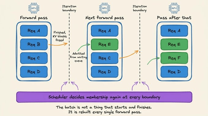
A finished sequence leaves at the next iteration boundary rather than at the end of the full batch run. And a waiting request enters at that same boundary. The batch is rebuilt every forward pass.

This, in itself, is not sufficient since rebuilding the batch every pass creates a problem of its own.

For instance, a request that’s prefilling 4,096 tokens together and a request decoding its 900th token don’t share a tensor shape, so there’s nothing to stack in the usual way.

Selective batching handles this, and it ensures that batching is applied only to the operations that can take it.

Every token scheduled in the step, whatever request it came from, is flattened into one long sequence of shape (total tokens*hidden size).

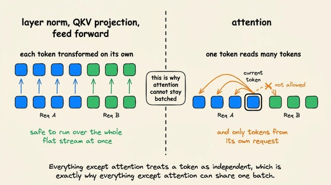
Layer norm, the QKV projections, and the feed-forward blocks all operate on each token independently, so they neither know nor care which request a token belongs to.

They run once across the whole flat stream at full efficiency.

But the attention operation can not work like this. A token may only attend to earlier tokens from its own request, and every request has a KV cache of a different length.

So the flat tensor is split at the attention boundary, attention runs separately for each request against that request’s own cache, and the outputs merge back into the stream before the next batched operation.

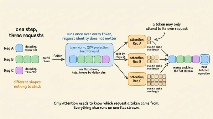
One scheduling step, clearly explained:

Between two forward passes the scheduler answers one question. Which requests run next, and how many tokens does each one get.

It answers that in four steps and we’ll use vLLM’s V1 scheduler as the reference implementation:

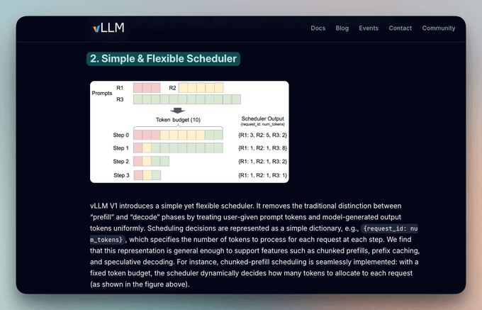
1. The scheduler fixes a budget for the step:

• max_num_batched_tokens caps the total tokens the step may issue

• and max_num_seqs caps how many sequences can be in flight at once.

2. Running requests get to claim compute budget first:

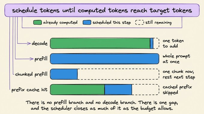
Each request carries a count of tokens already computed and a target count. The scheduler hands out tokens to reduce the gap between where a request currently is and where it wants to get to, spending from the budget as it goes.

A scheduler could reasonably keep two code paths here, one for prefill and one for decode, since prefill processes a whole prompt and decode produces a single token.

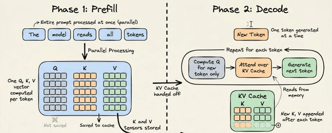
But in practice, there’s no such split. Prefill and decode look like different jobs, but the scheduler sees the same number.

It takes the target, subtracts what’s already computed, and hands out that many tokens if the budget allows:

So for a fresh 4,096 token prompt, that number is 4,096. For a request mid-generation, it’s 1. It’s the same line of code either way.

# simplified from vllm/v1/core/sched/scheduler.py

tokens_this_step = min(
    request.num_tokens_with_spec - request.num_computed_tokens,
    remaining_token_budget,
)

Chunked prefill and prefix caching need no extra handling either.

If a 4,096 token prompt doesn’t fit in the budget, the scheduler hands out 2,048 now and the other 2,048 in the next step.

If 3,000 of those 4096 tokens were already cached from an earlier request, only 1,096 are left to hand out.

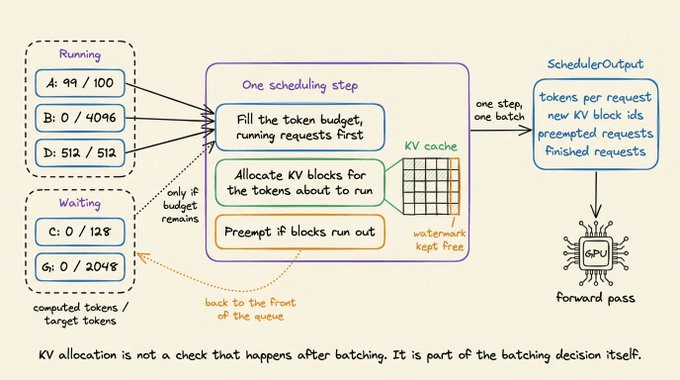
3. The scheduler claims KV blocks for the tokens it just assigned.

It reserves that memory while deciding, not after.

A step is only valid if the cache can hold what it produces, so when there aren’t enough free blocks, the scheduler takes them from the newest request in the running list.

4. Whatever budget is left goes to waiting requests

Requests that haven’t started yet get scheduled with whatever tokens are left over. If the running requests used the whole budget, nothing new starts this step.

The scheduler then hands the GPU a list of how many tokens each request runs and which KV blocks to write them into.

Token budget decides latency and throughput

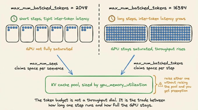
A step takes as long as the tokens inside it, which makes max_num_batched_tokens a latency setting as much as a throughput one.

To recall, max_num_batched_tokens is the total number of tokens the scheduler may put into one forward pass, added up across every request in the step. It isn’t a per request limit. A decoding request contributes one token, since one token is all it produces. A prefill contributes however many prompt tokens the scheduler hands it.

At around 2048 tokens, no step runs long, so inter-token latency stays tight and the GPU is often under-fed.

At around 16384, the GPU stays saturated and throughput rises, but every request in the batch waits out a longer step.

Size isn’t the only thing this budget setting controls.

With chunked prefill on, which is the V1 default wherever possible, the scheduler fills the budget with pending decodes first and gives what’s left to prefills, chunking a prefill that doesn’t fit.

Preemption

When block allocation fails, the scheduler frees a running request’s blocks, marks it preempted, resets num_computed_tokens to zero, clears its speculative tokens, and puts it back at the front of the waiting queue.

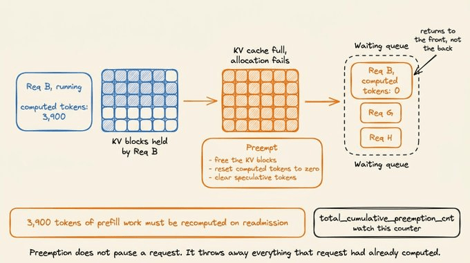
The reset to zero is an actual cost because, let’s say a request had already prefilled 3,900 tokens, and it then comes back with none of that saved, it must compute all 3,900 again.

V1 made recompute the default preemption mode and dropped the older swap path entirely.

From the outside, this looks like the GPU running out of headroom. Latency climbs as traffic rises, and adding replicas seems like the fix.

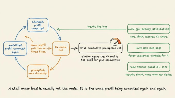
What’s actually happening is the same prefill being computed two or three times. Requests get preempted, readmitted, and preempted again, and every one of those cycles repeats work the GPU had already finished.

vLLM counts this in Prometheus as total_cumulative_preemption_cnt, and it’s the first metric to check when p99 climbs without a traffic change.

For context, p99 is the latency your slowest 1% of requests see. Averages hide preemption because most requests are never preempted, so problems show up in the tail.

Three settings improve it.

• Raise gpu_memory_utilization so more VRAM becomes KV cache

• Lower max_num_seqs so fewer sequences compete for it

• Raise tensor_parallel_size so weights shard across GPUs and leave more room per device.

Wrapping up

Everything above comes down to one loop.

The scheduler rebuilds the batch at every forward pass, hands out tokens against a fixed budget, and reserves KV blocks while it decides, and those three moves determine what your GPU actually produces.

Anyscale’s benchmark on OPT-13B found that as output lengths varied, static batching fell to around 81 tokens/s while vLLM reached 23x the throughput of naive Hugging Face serving on the same A100. None of that came from a faster model:

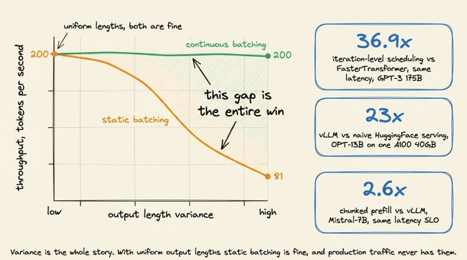
So if throughput or p99 is your problem, the scheduler is the layer to look at before the model.

The preemption counter is usually the cheapest place to start, since it tells you in one number whether your KV pool matches the concurrency you configured.

To dive deeper into the full LLMOps lifecycle, we have covered every bit of it in the LLMOps course, starting from fundamentals to production:

• Read Part 1 on fundamentals of LLMOps here →

• Read Part 2 on understanding the core building blocks of LLMs →

• Read Part 3 on the key components of LLMs, focusing on the attention mechanism, architectures like transformers and mixture-of-experts, and the fundamentals of pretraining and fine-tuning →

• Read Part 4 on decoding strategies, generation parameters, best practices, and the broader lifecycle of LLM-based applications →

• Read Part 5 on context + prompt engineering from a system perspective, in-context learning, types of prompts, and different prompting techniques →

• Read Part 6 on prompt versioning, defensive prompting, and techniques like verbalized sampling, role prompting, and more →

• Read Part 7 on context engineering, covering context types, context construction principles, and retrieval-centric techniques for building high-signal inputs →

• Read Part 8 on memory, dynamic, and temporal context in LLM systems, covering short and long-term memory, dynamic context injection, and common failure modes in agentic applications →

• Read Part 9 on evaluation methods and approaches for LLM-based applications, primarily focusing on building a strong understanding of the fundamental concepts →

• Read Part 10 on evaluation benchmarks in LLM applications, with task-specific methodologies, and the core tooling for evaluation of LLM apps →

• Read Part 11 on evaluation of multi-turn systems, tool use evaluations, tracing, and red teaming →

• Read Part 12 on LLM fine-tuning, parameter-efficient methods like LoRA and QLoRA, and alignment techniques such as RLHF, DPO, and GRPO →

• Read Part 13 on LLM inference optimization, KV caching, PagedAttention, FlashAttention, speculative decoding, and model parallelism →

• Read Part 14 on the fundamentals of LLM serving, including API-based access, inference with vLLM, and practical decisions.

👉 Over to you: what preemption counts do you see under peak load, and which knob moved them most?

Good day!