
Euclidean Distance vs. Mahalanobis Distance
Euclidean distance is not always useful.

From Models to Metal Mayhem @AWS re:Invent
If you are heading to AWS re:Invent and subscribed to DailyDoseofDS…
…then Bright Data is giving you an exclusive chance to watch the BattleBots live at the world‑famous arena in Las Vegas.

You’ll get to see live robots, real sparks, and Actual chaos.
Plus a room full of engineers, builders, and data people who like their systems…slightly destructive.
Daily Dose of DS subscribers get free access, but spots are limited.
👉 Claim your free BattleBots pass here →
Thanks to Bright Data for partnering today!
Euclidean Distance vs. Mahalanobis Distance
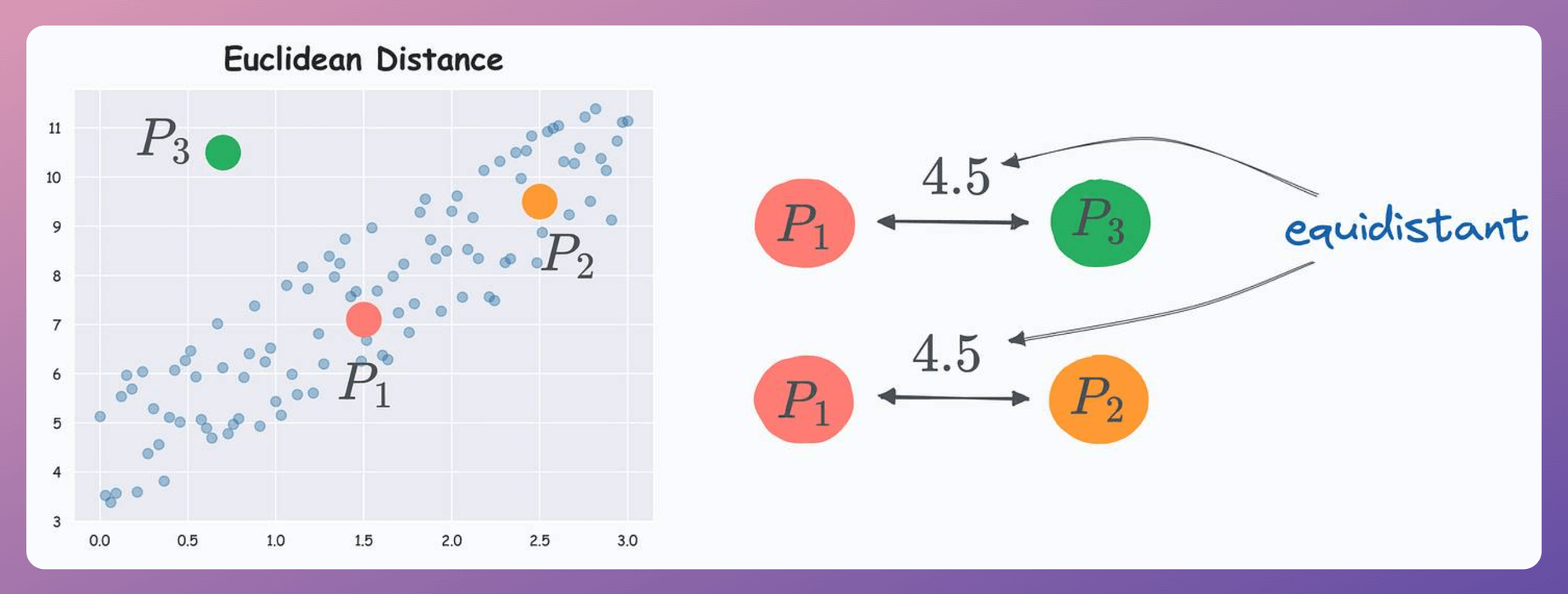
Consider the three points below in a dummy dataset with correlated features:

According to Euclidean distance, P1 is equidistant to P2 and P3.
But if we look at the data distribution, something tells us that P2 should be considered closer to P1 than P3 since P2 lies more within the data distribution.

Yet, Euclidean distance can not capture this.
Mahalanobis distance addresses this issue.
It is a distance metric that considers the data distribution during distance computation.
Referring to the above dataset again, with Mahalanobis distance, P2 comes out to be closer to P1 than P3:

How does it work?
The core idea is similar to what we do in Principal Component Analysis (PCA).
More specifically, we construct a new coordinate system with independent and orthogonal axes. The steps are:
Step 1: Transform the columns into uncorrelated variables.
Step 2: Scale the new variables to make their variance equal to 1.
Step 3: Find the Euclidean distance in this new coordinate system.
So, eventually, we do use Euclidean distance, but in a coordinate system with independent axes.
Uses
One of the most common use cases of Mahalanobis distance is outlier detection.
For instance, in this dataset, P3 is an outlier but Euclidean distance will not capture this.
But Mahalanobis distance provides a better picture:

Moreover, there is a variant of kNN that is implemented with Mahalanobis distance instead of Euclidean distance.
Further reading:
We covered 8 more pitfalls in data science projects here →
This mathematical discussion on the curse of dimensionality will help you understand why Euclidean produces misleading results in high dimensions.
👉 Over to you: What are some other limitations of Euclidean distance?
Cost complexity pruning in decision trees
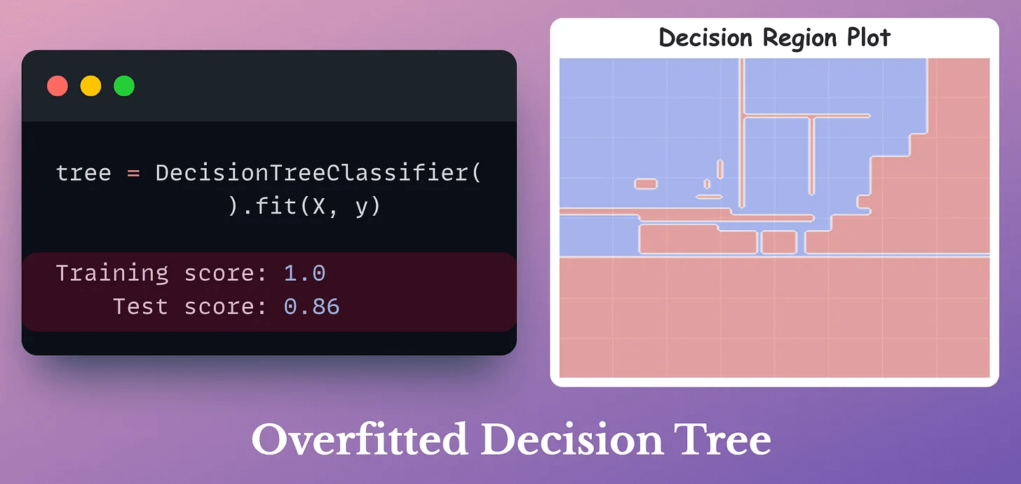
A decision tree can overfit any data because the algorithm greedily selects the best split at each node and is allowed to grow until all leaves are pure
For instance, consider this dummy dataset:
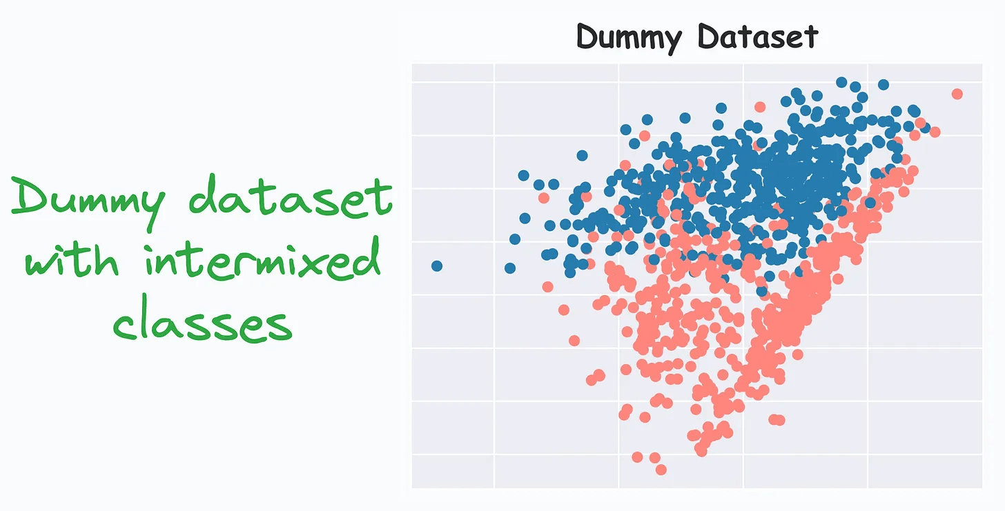
Fitting a decision tree on this dataset gives us the following decision region plot and results in 100% training accuracy:
Cost-complexity-pruning (CCP) is an effective technique to prevent this, which considers a combination of two factors for pruning a decision tree:
Cost (C): Number of misclassifications
Complexity (C): Number of nodes
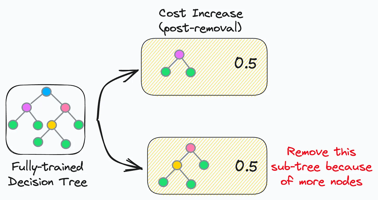
The idea is to iteratively drop sub-trees from a tree that lead to:
a minimal increase in classification cost
a maximum reduction of complexity (or nodes)
In other words, if two sub-trees lead to a similar increase in classification cost, then it is wise to remove the sub-tree with more nodes.
In sklearn, you can control cost-complexity-pruning using the ccp_alpha parameter:
large value of
ccp_alpha→ results in underfittingsmall value of
ccp_alpha→ results in overfitting
The objective is to determine the optimal value of ccp_alpha, which gives a better model.
Its effectiveness is evident from the image below:
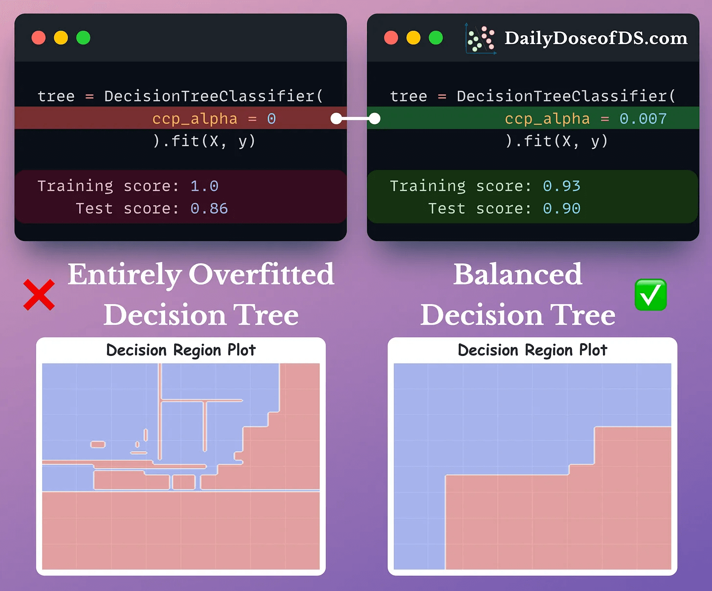
As depicted above, the CCP results in a much simpler and acceptable decision region plot.
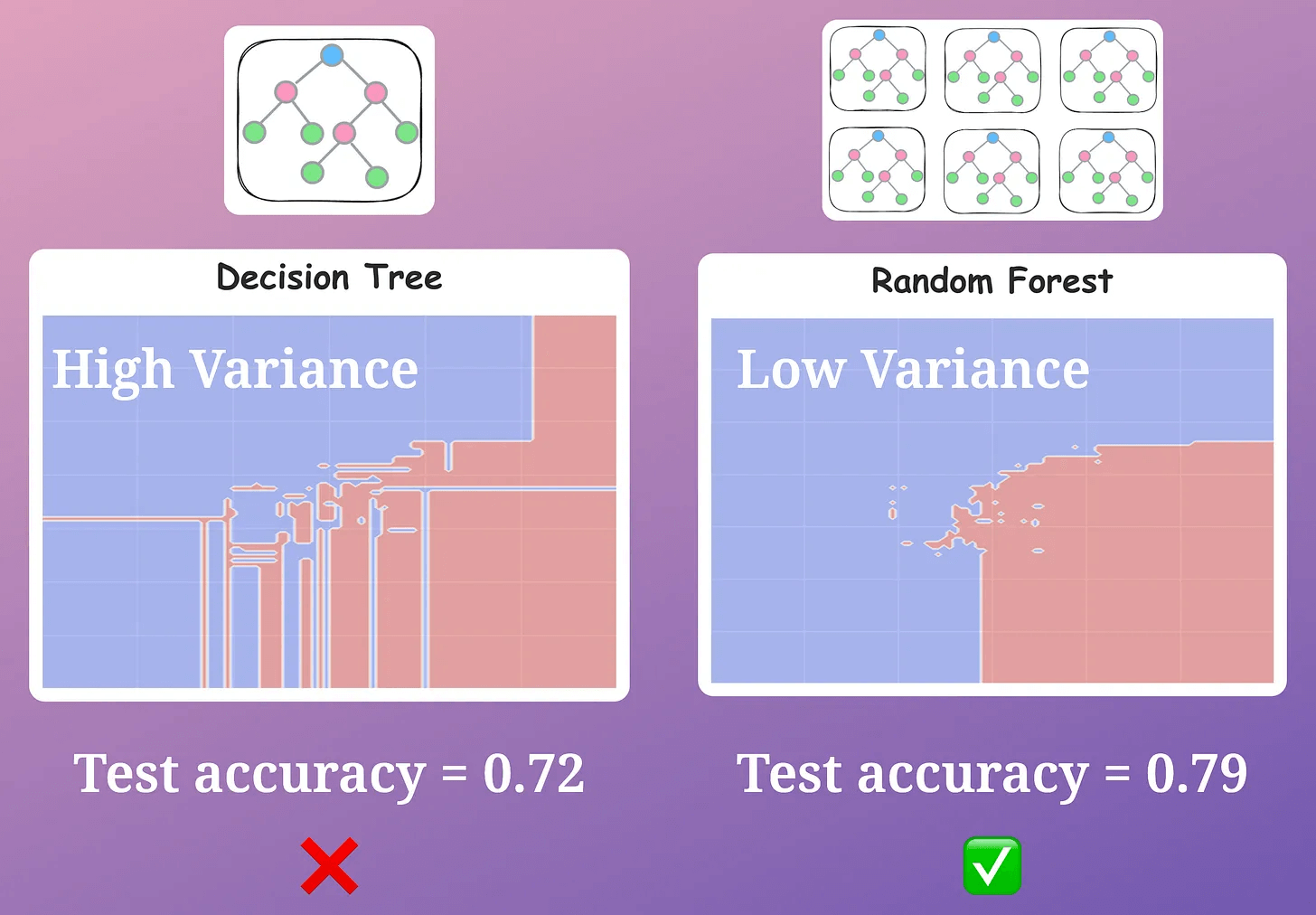
That said, Bagging is another pretty effective way to avoid this overfitting problem.
The idea is to:
create different subsets of data with replacement (this is called bootstrapping)
train one model per subset
aggregate all predictions to get the final prediction
As a result, it drastically reduces the variance of a single decision tree model, as shown below:
While we can indeed verify its effectiveness experimentally (as shown above), most folks struggle to intuitively understand:
Why Bagging is so effective.
Why do we sample rows from the training dataset with replacement.
How to mathematically formulate the idea of Bagging and prove variance reduction.
Can you answer these questions?
If not, we covered this in full detail here: Why Bagging is So Ridiculously Effective at Variance Reduction?

The article dives into the entire mathematical foundation of Bagging, which will help you:
Truly understand and appreciate the mathematical beauty of Bagging as an effective variance reduction technique
Why the random forest model is designed the way it is.
Also, talking about tree models, we formulated and implemented the XGBoost algorithm from scratch here: Formulating and Implementing XGBoost From Scratch.
It covers the entire mathematical details for you to learn how it works internally.
👉 Over to you: What are some other ways you use to prevent decision trees from overfitting?
Thanks for reading!
Spot on. This breakdown of Mahalanobis distance, especially how it handles correlated data like PCA, is super clear and makes a ton of sense for practical applications. Quick question though, for that second step where you scale the new varibles to make their variance equal, what's typically the preferred method you use for that part in practice?