Feature Discretization: An Underappreciated Technique for Model Improvement
Understanding the rationale behind a powerful yet overlooked technique in machine learning.
During model development, one of the techniques that many don’t experiment with is feature discretization.
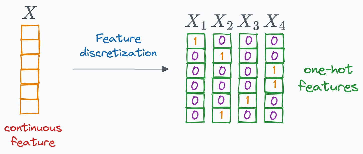
As the name suggests, the idea behind discretization is to transform a continuous feature into discrete features.
Why, when, and how would you do that?
Let’s understand this today.
Motivation for feature discretization
My rationale for using feature discretization has almost always been simple: “It just makes sense to discretize a feature.”
For instance, consider your dataset has an age feature:
In many use cases, like understanding spending behavior based on transaction history, such continuous variables are better understood when they are discretized into meaningful groups → youngsters, adults, and seniors.
For instance, say we model this transaction dataset without discretization.
This would result in some coefficients for each feature, which would tell us the influence of each feature on the final prediction.
But if you think again, in our goal of understanding spending behavior, are we really interested in learning the correlation between exact age and spending behavior?
It makes very little sense to do that.
Instead, it makes more sense to learn the correlation between different age groups and spending behavior.
As a result, discretizing the age feature can potentially unveil much more valuable insights than using it as a raw feature.
2 most common techniques for feature discretization
Now that we understand the rationale, there are 2 techniques that are widely preferred.
One way of discretizing features involves decomposing a feature into equally sized bins.
Another technique involves decomposing a feature into equal frequency bins:
After that, the discrete values are one-hot encoded.
One advantage of feature discretization is that it enables non-linear behavior even though the model is linear.
This can potentially lead to better accuracy, which is also evident from the image below:
A linear model with feature discretization results in a:
non-linear decision boundary.
better test accuracy.
So, in a way, we get to use a simple linear model but still get to learn non-linear patterns.
Isn’t that simple yet effective?
Another advantage of discretizing continuous features is that it helps us improve the signal-to-noise ratio.
Simply put, “signal” refers to the meaningful or valuable information in the data.
Binnng a feature helps us mitigate the influence of minor fluctuations, which are often mere noise.
Each bin acts as a means of “smoothing” out the noise within specific data segments.
Before I conclude, do remember that feature discretization with one-hot encoding increases the number of features → thereby increasing the data dimensionality.
And typically, as we progress towards higher dimensions, data become more easily linearly separable. Thus, feature discretization can lead to overfitting.
To avoid this, don’t overly discretize all features.
Instead, use it when it makes intuitive sense, as we saw earlier.
Of course, its utility can vastly vary from one application to another, but at times, I have found that:
Discretizing geospatial data like latitude and longitude can be useful.
Discretizing age/weight-related data can be useful.
Features that are typically constrained between a range makes sense, like savings/income (practically speaking), etc.
👉 Over to you: What are some other things to take care of when using feature discretization?
👉 If you liked this post, don’t forget to leave a like ❤️. It helps more people discover this newsletter on Substack and tells me that you appreciate reading these daily insights.
The button is located towards the bottom of this email.
Thanks for reading!
Latest full articles
If you’re not a full subscriber, here’s what you missed:
DBSCAN++: The Faster and Scalable Alternative to DBSCAN Clustering
Federated Learning: A Critical Step Towards Privacy-Preserving Machine Learning
You Cannot Build Large Data Projects Until You Learn Data Version Control!
Why Bagging is So Ridiculously Effective At Variance Reduction?
Sklearn Models are Not Deployment Friendly! Supercharge Them With Tensor Computations.
Deploy, Version Control, and Manage ML Models Right From Your Jupyter Notebook with Modelbit
Gaussian Mixture Models (GMMs): The Flexible Twin of KMeans.
To receive all full articles and support the Daily Dose of Data Science, consider subscribing:
👉 Tell the world what makes this newsletter special for you by leaving a review here :)
👉 If you love reading this newsletter, feel free to share it with friends!


You wouldn't want to do this when using a tree-based model, right? There is a lot of information lost from binning, and the learning algorithm can't find the best split points in the original data.
I can see the utility for a linear model, as we are getting additional degrees of freedom and we can inject domain knowledge, but the split points should be meaningful.
Still over my head, but beginning to see patterns. Thanks love the learning aspect, so much appreciated.