

In today’s newsletter:
Build a semantic search inside your database without an embedding pipeline.
8 LLM precision formats.
6 memory optimization techniques for Agentic systems.
[Hands-on] Build semantic search inside your database without an embedding pipeline
We typed a plain English query against 21,000 movie plots and got back semantically relevant results without writing a single line of embedding code.
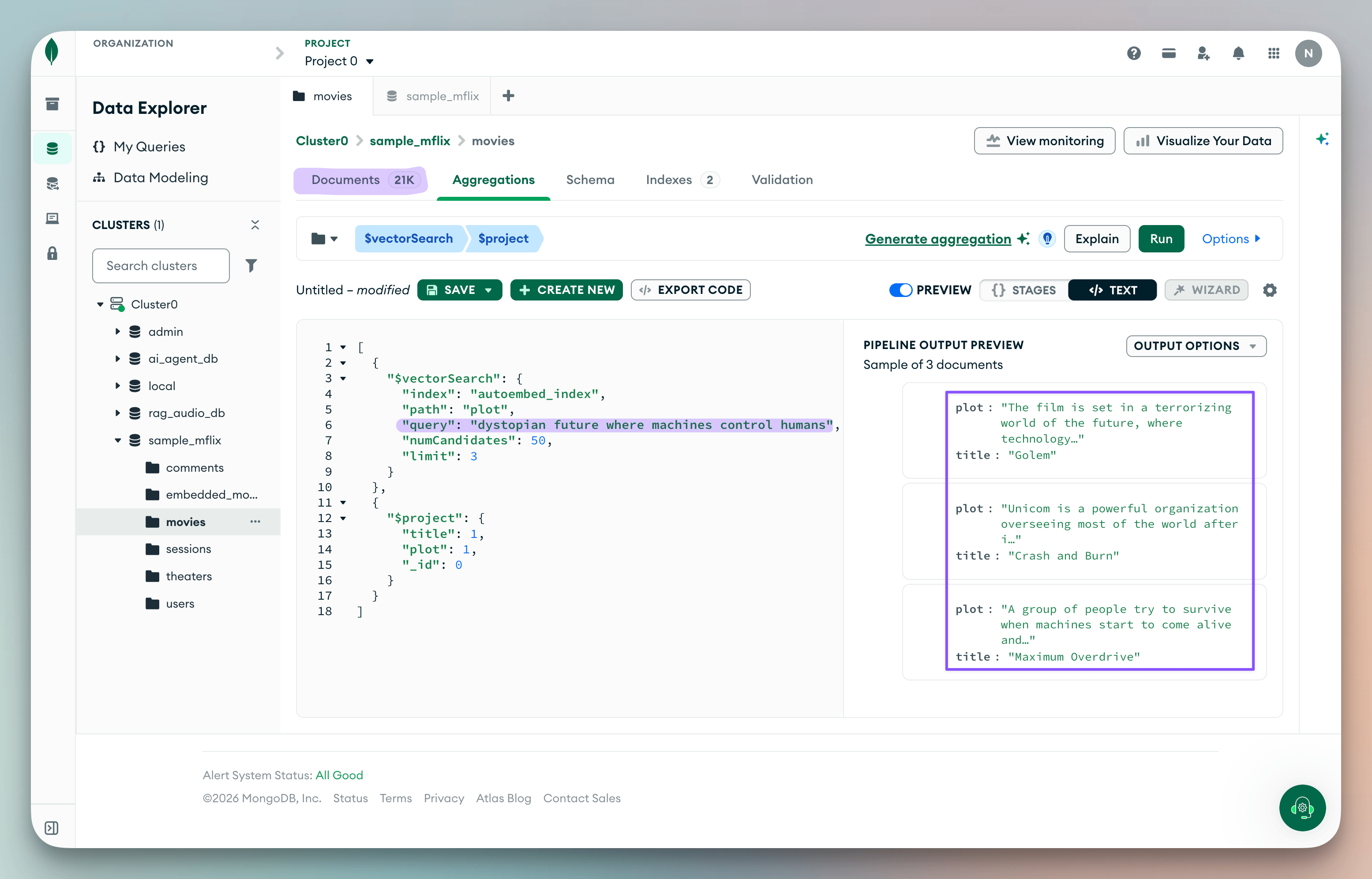
The database is MongoDB Atlas, which added auto-embedding powered by Voyage AI directly into its vector search index configuration.
When you add semantic search to an app, the standard move is to wire up an external embedding service, sync vectors to a separate store, and write glue to keep everything updated as data changes.
Most teams never question this setup because that’s just how the stack looked when vector search was new.
The real problem shows up later when your data changes, but your pipeline has already run, and search quality starts degrading in ways that are hard to pin down because nothing is explicitly broken.

MongoDB Atlas handles this with auto-embedding. You point an index at a text field, specify a Voyage AI model, and it generates and maintains the vectors inside the database.
When a document changes, it re-embeds automatically, so your search stays current.
Setting up auto-embedding
Load MongoDB’s sample dataset from your Atlas cluster and navigate to sample_mflix → movies. Then go to Search & Vector Search → Create Search Index.
On the index creation screen:
Select Vector Search as the search type
Scroll down and select Automated Embedding under “How do you want to set up your vector data?”
Name your index
autoembed_indexSelect
sample_mflix→moviesas the database and collectionChoose JSON Editor as the configuration method
Atlas pre-populates the config. Just replace <field-name> with plot:
{
  "fields": [
    {
      "type": "autoEmbed",
      "modality": "text",
      "path": "plot",
      "model": "voyage-4"
    }
  ]
}
Once the index flips to Active, open the Aggregation tab on the movies collection and run:
[
  {
    "$vectorSearch": {
      "index": "autoembed_index",
      "path": "plot",
      "query": "dystopian future where machines control humans",
      "numCandidates": 50,
      "limit": 3
    }
  },
  {
    "$project": {
      "title": 1,
      "plot": 1,
      "_id": 0
    }
  }
]
The results come back with movies whose plots share none of those exact words with the query, which is the index doing semantic matching rather than keyword lookup.
One index config replaced the embedding service, the vector store, and the sync layer you used to maintain separately.
If you want to go deeper, MongoDB has a full AI Skill Badges program on MongoDB University covering everything from vector search fundamentals to agentic memory and RAG, and each badge earns a Credly credential you can share on LinkedIn.
Thanks to MongoDB for working with us on today’s issue!
8 LLM precision formats
A 12GB consumer GPU cannot hold a 7B model in FP32, which needs 28GB just for the weights.
But running ollama run llama3 on that card works anyway.
The reason is that Ollama does not ship weights in FP32.
Instead, it pulls a Q4_K_M GGUF by default, which averages around 4.8 bits per weight and puts a 7B model near 4.1GB.
We covered several different LLM quantization techniques here →
Every format below FP32 is doing the same thing, i.e., trading numeric detail for memory.
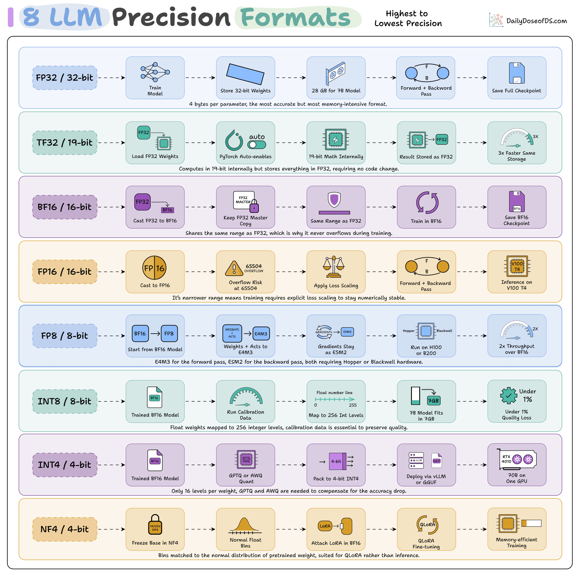
The visual below explains 8 such LLM precision formats:
Before we dive into them, some background:
A floating-point number splits its bits three ways.
One sign bit, then exponent bits that decide how large or small a value can get, then mantissa bits that decide how finely values can be told apart inside that range.
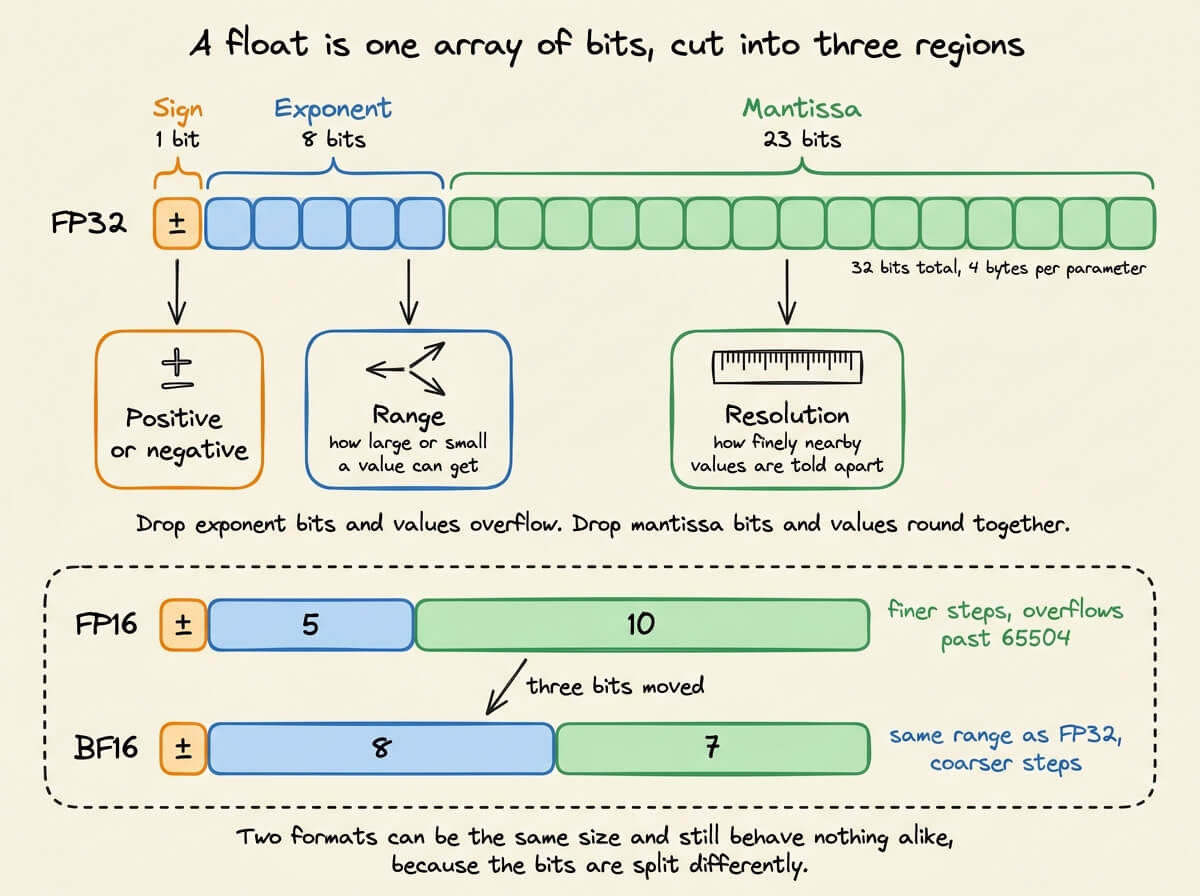
Cutting exponent bits causes overflow, where large values saturate, and training blows up.
Cutting mantissa bits causes rounding error, where nearby values collapse into the same number and the error accumulates.
Different formats focus on different sides.
1) FP32 has 8 exponent bits and 23 mantissa bits, reaching about 3.4e38.
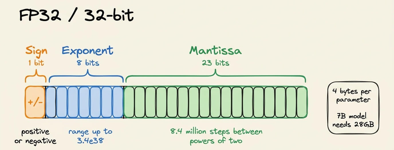
Four bytes per parameter is expensive, but optimizer states and master weights still use FP32 even in low-precision training runs, because the gradient updates are small enough that FP16 storage might round them away entirely.
2) TF32 is 19 bits, made of FP32’s 8 exponent bits and FP16’s 10 mantissa bits.
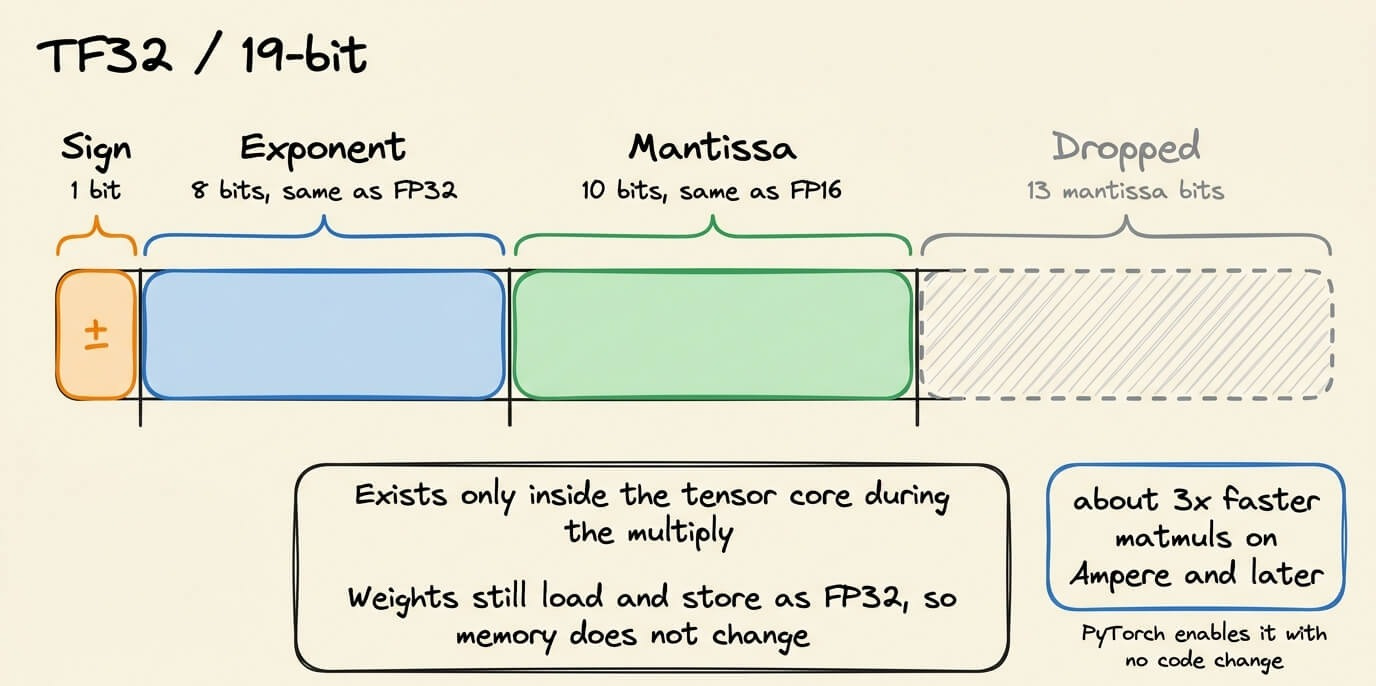
It only exists inside the tensor core, so weights load and store as FP32, and memory usage does not drop at all.
PyTorch enables it on Ampere and later without any code change, and this small change results in roughly 3x faster matmuls in exchange for 13 fewer mantissa bits during the multiplication process.
3) BF16 keeps FP32’s 8 exponent bits and cuts the mantissa to 7.
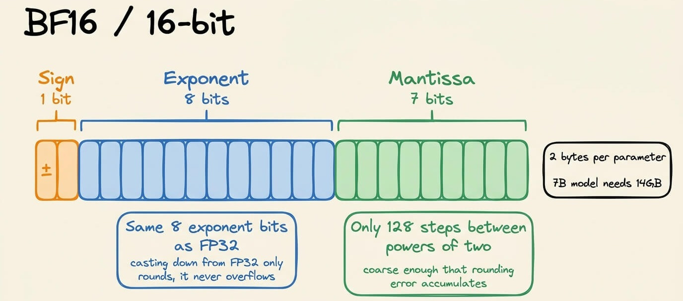
An identical range means casting down from FP32 only rounds and never overflows, which is why it has become the pre-training default.
4) FP16 splits the same 16 bits the other way, 5 exponent bits and 10 mantissa bits.
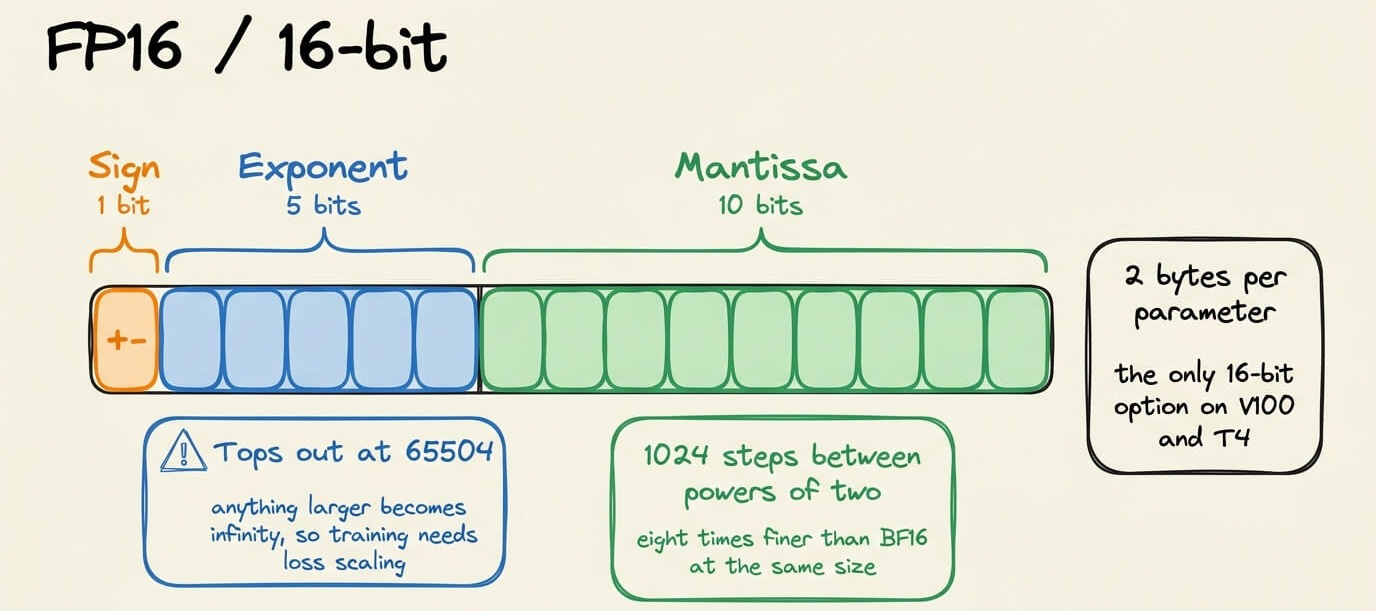
It resolves values eight times more finely than BF16 but is limited to just 65504, so gradients above that become infinity, and training needs loss scaling to survive.
It is also the only 16-bit option on V100 and T4 class hardware, which predate BF16.
An RL fine-tuning paper from late 2025 found BF16’s rounding error accumulates across autoregressive sampling until the training and inference engines assign different probabilities to the same tokens, and that moving the whole pipeline to FP16 removed the divergence.
5) FP8 has two layouts:
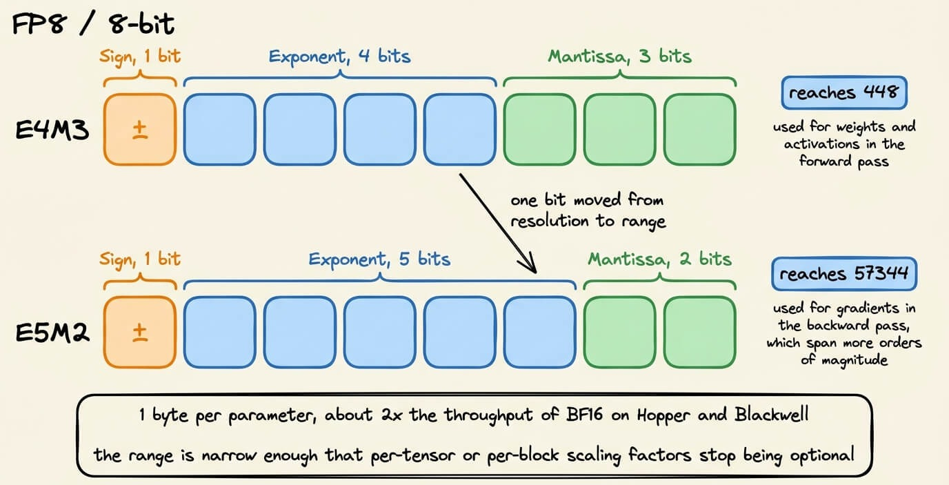
E4M3 reaches 448 and is ideal for weights and activations
E5M2 reaches 57344 and is ideal for gradients, which span more orders of magnitude.
Throughput-wise, this is about 2x faster BF16, but since the range is narrow, scaling factors per tensor or per block are no longer optional.
6) INT8 has no floating point.
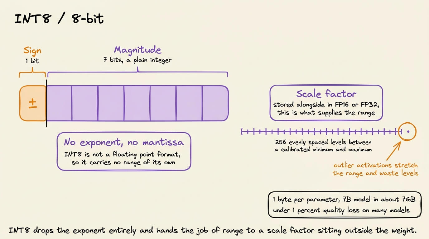
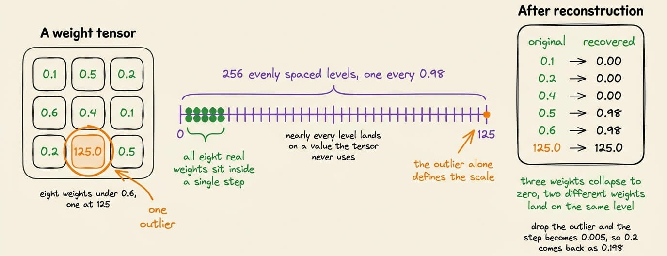
Weights map onto 256 evenly spaced integer levels between a calibrated minimum and maximum, which puts a 7B model in about 7GB with under 1% quality loss on many models.
Yes, even spacing is indeed a weakness, since a few outlier activations stretch the range and waste levels on values almost nothing uses.
7) INT4 gives each weight 16 possible values:
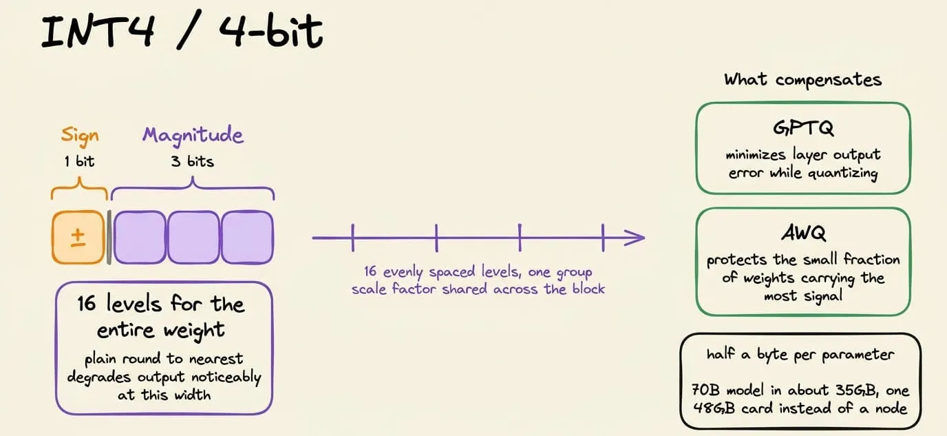
To compare, INT8 can take 256 values, so the gaps between allowed values are sixteen times wider, and every weight moves further when it snaps to the nearest one.
Rounding to the nearest value keeps that individual move as small as possible. But a layer multiplies thousands of weights against the input and adds the results, so the error that shows up in the output is the sum of thousands of these moves.
Rounding cannot see that sum. It treats every weight as equally important, when in practice, only some of them meaningfully change the output.
GPTQ works around this by quantizing a block one weight at a time and adjusting the weights not yet done to cancel the error already made.

AWQ finds the channels carrying the most signal and scales them up before quantizing, spending more of the 16 values where it counts.

Both need calibration data, a few hundred real inputs, since that is the only way to tell which weights matter.
8) NF4 also uses 16 levels but spaces them unevenly, with bin edges placed along a normal distribution because pretrained weights sit close to a zero-centered Gaussian.
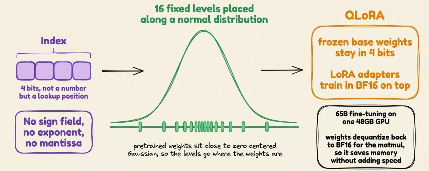
It exists for QLoRA, where the base model stays frozen in 4 bits, and LoRA adapters train in BF16 on top, which puts 65B fine-tuning on one 48GB GPU at 16-bit task quality.
The weights get dequantized back to BF16 for the actual matmul, so it saves memory without adding speed.
As a result, quality degrades far less on larger models, so a 70B at 4-bit generally beats a 13B at 16-bit for the same memory.
And the sharp drop is between 3-bit and 4-bit, not between 4-bit and 8-bit, which is why 4-bit ended up as the default everywhere from Ollama to vLLM.
To dive deeper, we have already written a full deep dive on Quantization, specifically, which covers several of these methods with their simplified mathematics.
Learn how Quantization optimizes LLMs to run them on tiny hardware here →
6 memory optimization techniques for Agentic systems
We recently added Part 16 and Part 17 to our AI Agents crash course, where we use LangGraph to implement 6 production-grade memory optimization techniques in agentic workflows.
But what exactly is Memory, and why is it so powerful for Agentic systems?
To understand this, consider an Agentic system without Memory (below):

In iteration #1, the user mentions their favorite color.
In iteration #2, the Agent knows nothing about iteration #1.
This means the Agent is mostly stateless, and it has no recall abilities.
But now consider an Agentic system built with Memory (below):

In iteration #1, the user mentions their favorite color.
In iteration #2, the Agent can recall iteration #1.
Memory matters because if a memory-less Agentic system is deployed in production, every interaction with that Agent will be a blank slate.

It doesn’t matter if the user told the Agent their name five seconds ago, it’s forgotten. If the Agent helped troubleshoot an issue in the last session, it won’t remember any of it now.
With Memory, your Agent becomes context-aware and practically applicable.
But Memory isn’t an abstract concept.
If you dive deeper, it follows a structured and intuitive architecture with several types of Memory.
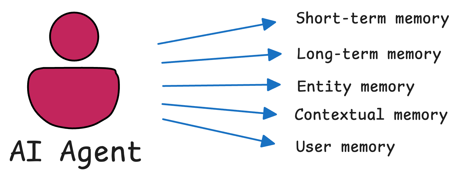
Short-Term Memory
Long-Term Memory
Entity Memory
Contextual Memory, and
User Memory
Each serves a unique purpose in helping agents “remember” and utilize past information.
To simulate memory, the system has to manage context explicitly: choosing what to keep, what to discard, and what to retrieve before each new model call.
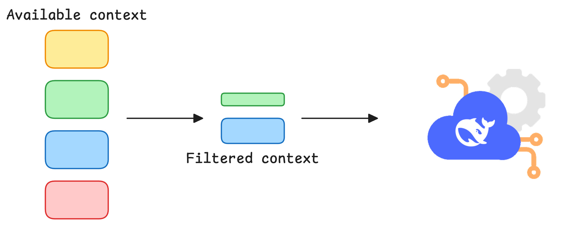
This is why memory is not a property of the model itself. It is a system design problem that can also be optimized, and we covered them in these two parts:
Also, Part 8 and Part 9 of the crash course cover memory with CrewAI:
Both parts cover:
5 types of Memory from a theoretical, practical, and intuitive perspective.
How each type of Memory helps an Agent.
How an Agent retrieves relevant details from the Memory.
The underlying mechanics of Memory and how it is stored.
How to utilize each type of Memory for Agents (implementations).
How to customize Memory settings.
How to reset the Memory if needed.
And more.
Happy learning!