How to Achieve 2.8x Faster Automatic Speech Recognition

...based on how production voice systems are built.

Dependency monitoring for all codebases

External services are peppered throughout your code: talking to APIs, auth providers, payment processors, etc.

Coding agents make it worse, because while the code works, nobody has a clear inventory of what it depends on or whether those dependencies are healthy.

And vendors never report outages fully nor in a quick fashion.

Gloria.dev’s first tool, Canary, solves this by providing you with a global monitoring layer.

It scans the codebase to discover every internal and external dependency, turns each one into an authenticated health check, and runs those checks on a schedule. Outages, error spikes, and cost anomalies surface before they reach users.

The dependency inventory stays current automatically, driven by the code itself rather than a manually maintained list.

And it’s free.

Learn more about Gloria.dev here →

Thanks to the team for partnering today!

---

How to achieve 2.8x faster automatic speech recognition

Speech recognition systems typically spend more compute processing silence than they spend processing speech. And it’s not something a bigger model fixes.

Consider talking to a voice agent and pausing mid-sentence. “I want to book a... uhh... table for two, around... 7pm?”

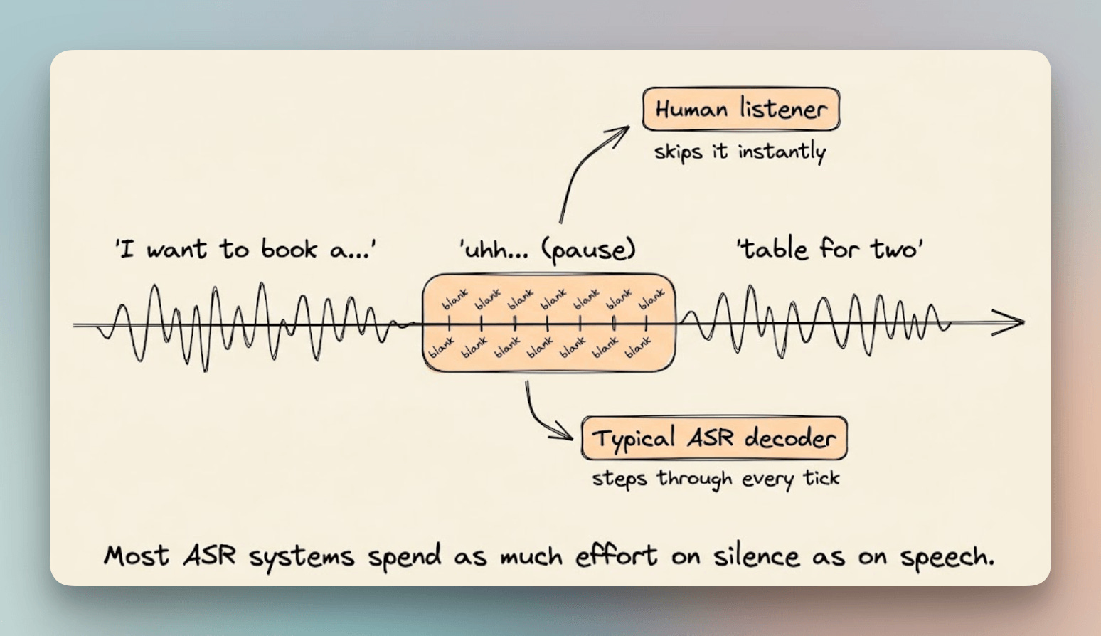
A human listener tunes out the silence and the “uhh” instantly, but automatic speech recognition (ASR) systems usually process that dead air piece by piece, the same way they process actual speech.

If voice agents feel laggy, this is part of why.

For a 10-second audio clip, a typical speech decoder runs about 125 sequential calls, most of them spent confirming that nothing new happened.

That decoder, called an RNN-Transducer (RNN-T), is the dominant architecture in production ASR today.

Why RNN-T wastes most of its steps

A frame is a thin slice of audio, just a few milliseconds wide. RNN-T processes these one at a time.

At every frame, a small network called the joint network looks at that slice plus everything predicted so far, and outputs a probability distribution over the vocabulary plus one special token called blank.

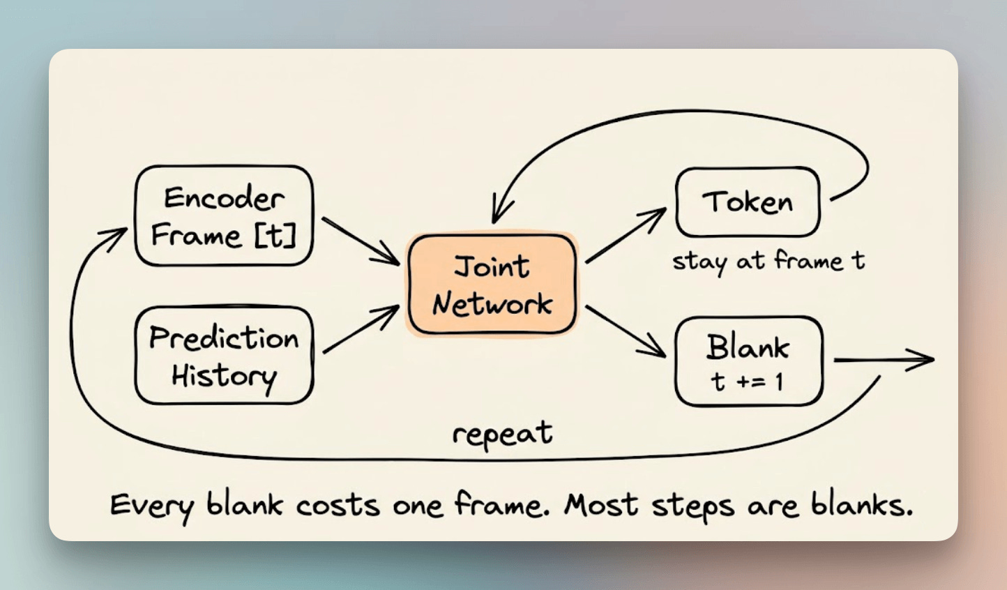
If the model picks blank, the frame counter advances by one. If it picks a real token like “the” or “cat,” the token gets added to the output, and the frame counter stays put until the next blank.

So across those 125 steps, most of the calls land on silence, pauses, held phonemes, the “uhh” before “table for two,” stepped through one blank at a time.

The joint network itself is cheap, often just a linear layer. What’s expensive is that you can’t skip ahead.

Each call depends on the previous output, so the calls are strictly sequential and can’t be parallelized.

This compounds on longer audio, where a 60-second call has roughly six times the decoder steps of a 10-second clip, and most of those extra steps are still just blank.

What frame-skipping should look like

A bigger encoder or more training data is not the solution to this, and word error rate (WER) alone is the wrong thing to optimize for, because it says nothing about speed.

A model that’s marginally more accurate but takes 10 seconds to transcribe 1 second of audio is useless in a real-time system.

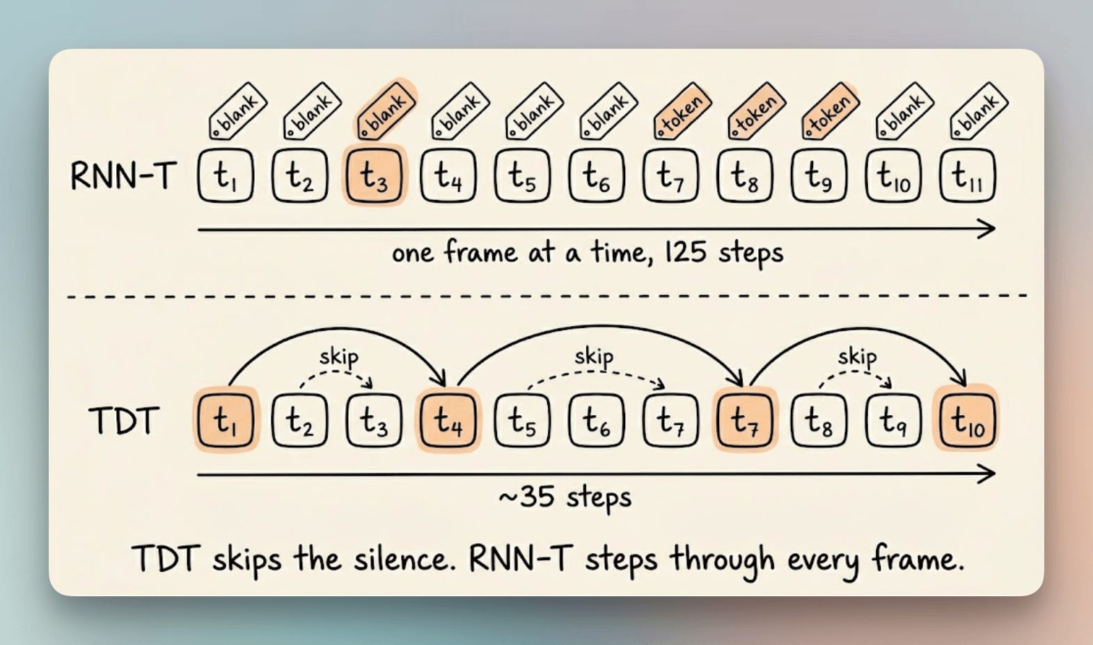
The fix is letting the decoder predict its own stride, how many frames to skip, not just what token to emit.

If the model already knows a stretch of audio is silence, it should jump past all of it in one step instead of confirming “still nothing” 6 times in a row.

Speechmatics (a real-time speech-to-text API used in production voice agents) actually implements exactly this approach, using their Token-and-Duration Transducer (TDT).

It’s the same architecture behind NVIDIA’s Parakeet TDT models, which led the Huggingface Open ASR Leaderboard on throughput despite using the same encoder size and training data as plain RNN-T models ranked below them on that same leaderboard.

The entire gap comes from this one decoder-level change.

How TDT works

The Token-and-Duration Transducer (TDT) keeps the encoder and prediction history network completely unchanged.

The only modification is a second output head on the joint network.

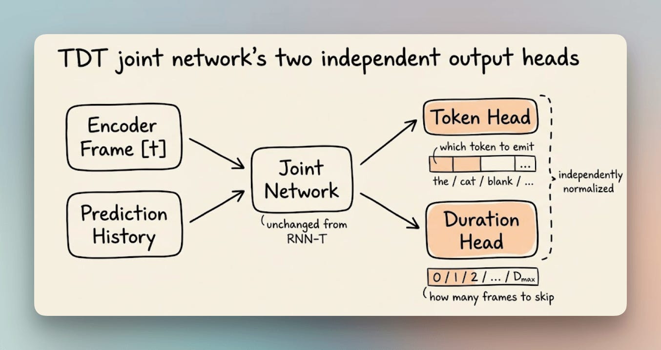
The original joint network has a single output, a distribution over the vocabulary plus blank. TDT’s joint network has two independent outputs:

• Token distribution: the same as before, predicting which token to emit

• Duration distribution: over a predefined set of values (commonly 0 through 4), predicting how many frames that step covers

So instead of always advancing by exactly 1 frame, the model now predicts its own stride.

If it predicts a duration of 4, the frame counter jumps forward 4 steps. The model learned during training that those 4 frames were going to be blank anyway.

Here’s what the decoding loop looks like:

# TDT Greedy Decoding (simplified)
t = 0
output = []
while t < T:
    token_logits, duration_logits = joint(encoder[t], predictor(output))
    token = argmax(token_logits)
    duration = argmax(duration_logits)

    if token == BLANK:
        t += max(duration, 1)  # blanks must advance at least 1 frame
    else:
        output.append(token)
        t += duration          # tokens can have duration=0 (no frame advance)

Blanks and tokens handle frame advancement differently.

Blanks must advance at least 1 frame, otherwise decoding would stall on silence. Tokens can have duration=0, meaning the model emits a token and stays on the same frame, useful for fast speech where multiple tokens align to a single frame.

Why are the two heads independent?

The obvious alternative is predicting token and duration jointly, but that explodes the output space.

A joint distribution over every token-duration combination would have vocabulary size × number of duration buckets possible outcomes.

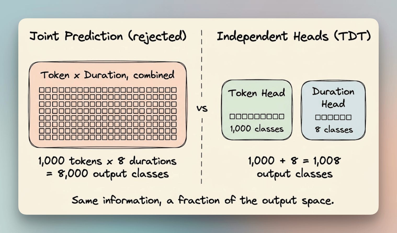
Take a vocabulary of 1,000 tokens with a hypothetical 8 duration buckets, that’s 8,000 output classes instead of 1,008.

This leads to a larger output space, which is harder to train, and the added precision rarely helps because token identity and frame coverage are mostly unrelated.

Keeping them independent means each head has a small, clean output space without interfering with the other’s gradients.

Training still uses the same algorithm as RNN-T, with the lattice now allowing multi-frame transitions instead of single-frame ones.

The benchmarks

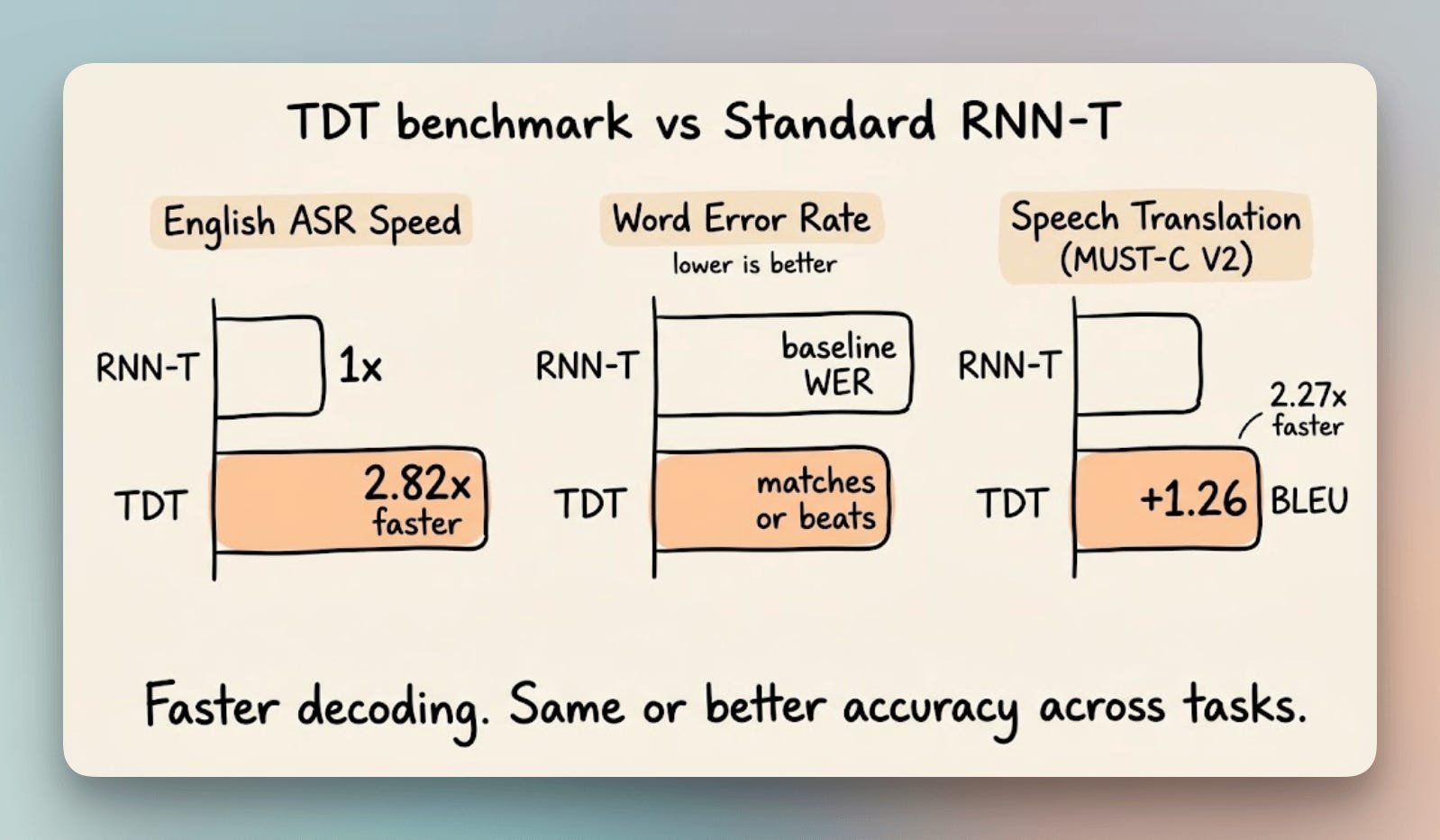
On English ASR, TDT matches or beats standard RNN-T on word error rate while decoding up to 2.82x faster.

The gains carry across tasks. On speech translation (MUST-C V2), TDT picks up 1.26 BLEU points, a standard translation accuracy metric, over RNN-T while running 2.27x faster.

The gains are largest on longer audio and silence-heavy recordings, exactly where blank-heavy decoding costs the most.

This is why Parakeet TDT models sit at the top of the Huggingface Open ASR Leaderboard on RTFx, the metric for how many seconds of audio a model processes per second of wall-clock time.

Putting it together

The encoder processes the whole audio clip at once, in parallel, before decoding even starts.

That part never changes with TDT.

All the savings are in the decoder, the part that has to run one step at a time. Each joint network call depends on the previous prediction, so those calls can’t be parallelized.

Cutting that call count by 2.82x translates directly to wall-clock time, which is why TDT-based models lead on RTFx while models with marginally better WER sit below them.

The full change from RNN-T to TDT is one extra output head on the joint network, with the encoder and loss structure staying identical.

Speechmatics runs exactly this in production. Their API scored 1.07% pooled WER on the Pipecat voice agent benchmark across 1,000 samples.

You can read the full technical breakdown from Speechmatics here →

---

AI Agent deployment strategies!​

Deploying AI agents isn’t one-size-fits-all. The architecture you choose can make or break your agent’s performance, cost efficiency, and user experience.

Here are the 4 main deployment patterns you need to know:

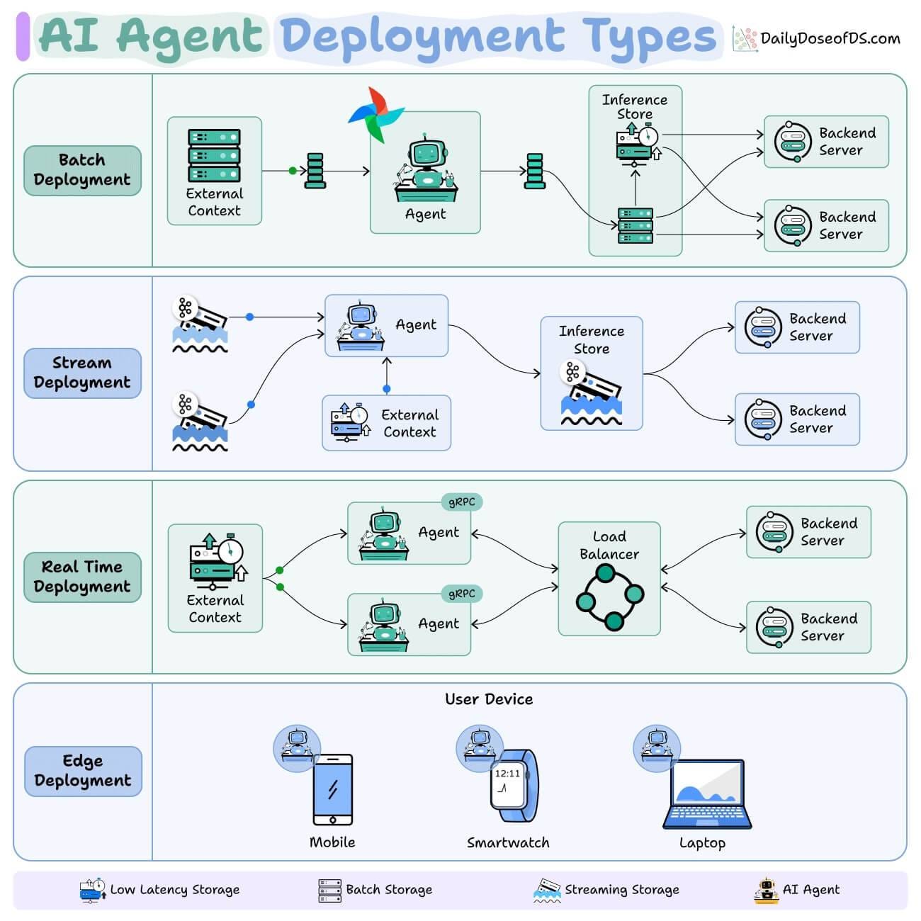
1) Batch deployment

You can think of this as a scheduled automation.

• The Agent runs periodically, like a scheduled CLI job.

• Just like any other Agent, it can connect to external context (databases, APIs, or tools), process data in bulk, and store results.

• This typically optimizes for throughput over latency.

• This is best for processing large volumes of data that don’t need immediate responses.

2) Stream deployment

Here, the Agent becomes part of a streaming data pipeline.

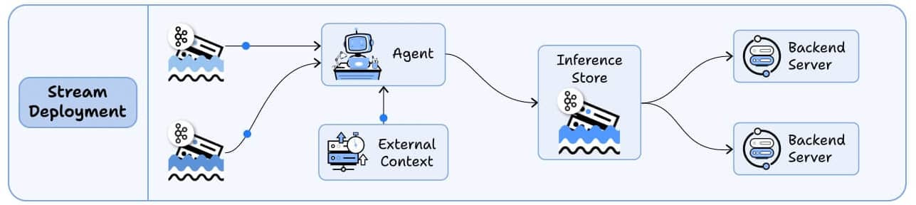
• It continuously processes data as it flows through systems.

• Your agent stays active, handling concurrent streams while accessing both streaming storage and backend services as needed.

• Multiple downstream applications can then make use of these processed outputs.

• Best for: Continuous data processing and real-time monitoring

3) Real-Time deployment

This is where Agents act like live backend services.

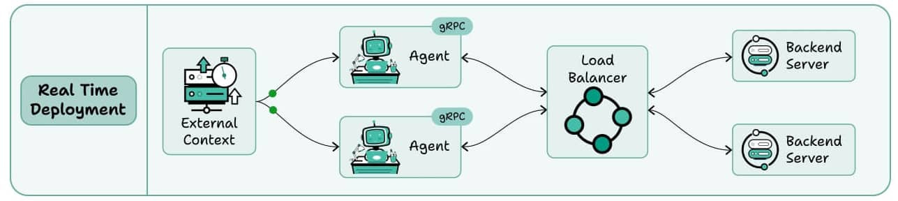
• The Agent runs behind an API (REST or gRPC).

• When a request arrives, it retrieves any needed context, reasons using the LLM, and responds instantly.

• Load balancers ensure scalability across multiple concurrent requests.

• This is your go-to for chatbots, virtual assistants, and any application where users expect sub-second responses.

4) Edge deployment

The agent runs directly on user devices: mobile phones, smartwatches, and laptops, so no server round-trip is needed.

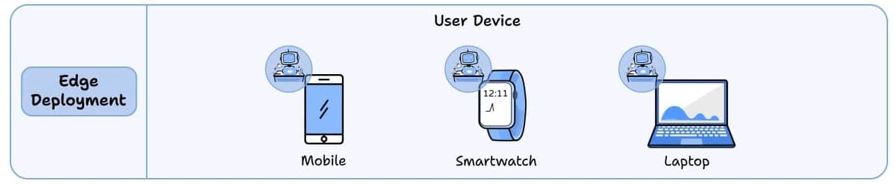
• The reasoning logic lives inside your mobile, smartwatch, or laptop.

• Sensitive data never leaves the device, improving privacy and security.

• Useful for tasks that need to work offline or maintain user confidentiality.

• Best for: Privacy-first applications and offline functionality

---

To summarize:

• Batch = Maximum throughput

• Stream = Continuous processing

• Real-Time = Instant interaction

• Edge = Privacy + offline capability

Each pattern serves different needs. The key is matching your deployment strategy to your specific use case, performance requirements, and user expectations.

We’ll have already covered deployment extensively in the LLMOps course:

• ​Read Part 1 on fundamentals of LLMOps here →​

• ​Read Part 2 on understanding the core building blocks of LLMs →​

• ​Read Part 3 on the key components of LLMs, focusing on the attention mechanism, architectures like transformers and mixture-of-experts, and the fundamentals of pretraining and fine-tuning →​

• ​Read Part 4 on decoding strategies, generation parameters, best practices, and the broader lifecycle of LLM-based applications →​

• ​Read Part 5 on context + prompt engineering from a system perspective, in-context learning, types of prompts, and different prompting techniques →​

• ​Read Part 6 on prompt versioning, defensive prompting, and techniques like verbalized sampling, role prompting, and more →​

• ​Read Part 7 on context engineering, covering context types, context construction principles, and retrieval-centric techniques for building high-signal inputs →​

• ​Read Part 8 on memory, dynamic, and temporal context in LLM systems, covering short and long-term memory, dynamic context injection, and common failure modes in agentic applications →​

• ​Read Part 9 on evaluation methods and approaches for LLM-based applications, primarily focusing on building a strong understanding of the fundamental concepts →​

• ​Read Part 10 on evaluation benchmarks in LLM applications, with task-specific methodologies, and the core tooling for evaluation of LLM apps →​

• ​Read Part 11 on evaluation of multi-turn systems, tool use evaluations, tracing, and red teaming →​

• ​Read Part 12 on LLM fine-tuning, parameter-efficient methods like LoRA and QLoRA, and alignment techniques such as RLHF, DPO, and GRPO →​

• ​Read Part 13 on LLM inference optimization, KV caching, PagedAttention, FlashAttention, speculative decoding, and model parallelism →​

• ​Read Part 14 on the fundamentals of LLM serving, including API-based access, inference with vLLM, and practical decisions.​

👉 Over to you: What deployment pattern are you using for your AI agents? Or are you combining multiple approaches?

Good day!