
How to Beat GRPO Without Touching Model Weights
Berkeley beat GRPO by 10 points with 35× fewer rollouts and no GPU training,

A tricky LLM interview question for AI Engineers

You’re fine-tuning a model for Python code generation. The data was generated using the strongest LLMs like Opus/GPT.
But the fine-tuned model performs better when you use a weaker teacher instead.
Why did this happen?
A stronger teacher model can produce worse fine-tuning results. This sounds counterintuitive, but it is a well-documented effect in knowledge distillation research.
Large models solve a basic problem using abstractions, type hints, and patterns.
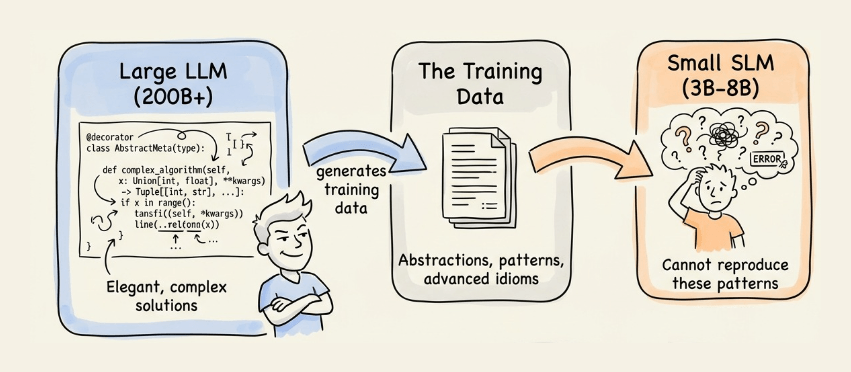
A Qwen3-8B model does not have enough capacity to reproduce those patterns. So instead of learning clean solutions, it learns an approximation of something it cannot fully represent.
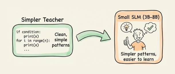
However, a weaker teacher solves the same problem correctly, but with simpler patterns that the student can actually replicate.
A recent paper from Fastino Labs also documented this.
The researchers used Pioneer, their fine-tuning agent that takes a task description, generates training data, selects a base model, runs experiments, and iterates until the model hits a performance target, all without human intervention.
During one of those runs, Pioneer fine-tuned Qwen3-8B on Python code generation.
The agent tried two different teacher models for synthetic data generation: one large frontier model and one smaller model.
The frontier model’s data hurt performance.
The smaller model’s data performed much better in fewer iterations.
And the fine-tuning Agent was smart enough to catch this behavior. It measured the results from both teachers, saw that the frontier model was making things worse, and dropped it.
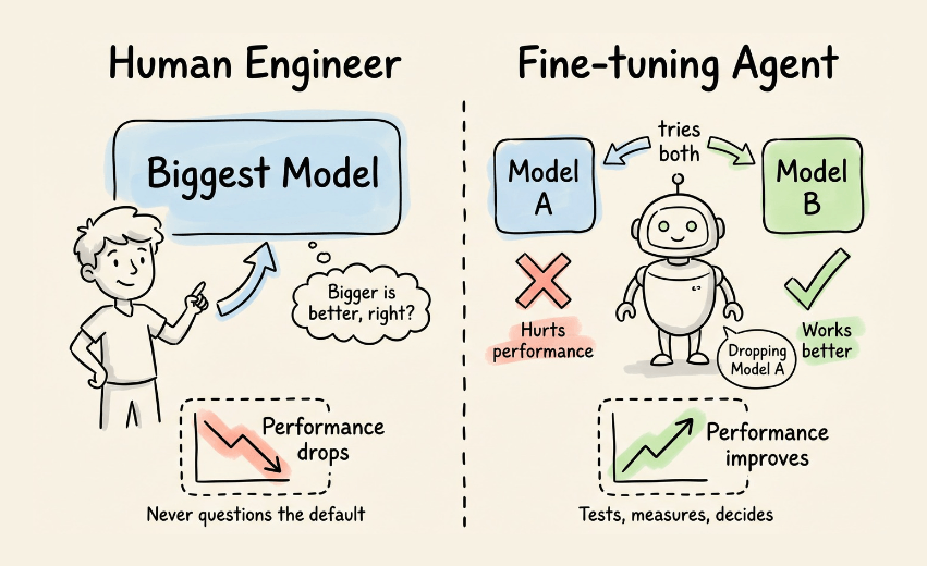
A human engineer would likely have defaulted to a bigger model because it is the stronger model, and might not have questioned that choice.
The paper explains three reasons this happens:
→ Capacity mismatch: The student cannot learn the teacher’s internal representations when the gap is too large. Increasing teacher size first helps, then hurts beyond a certain point.
→ Forgetting pretrained knowledge: Qwen3-8B already knows how to write Python from pretraining. Fine-tuning on a complex coding style from a much larger model can overwrite that existing capability.
→ Over-complexity in training data: A large model will solve “reverse a linked list” with elegant abstractions and comprehensive error handling. That is correct code, but it is also unnecessary complexity for the task. A simpler teacher generates solutions that match the task’s actual complexity, and the student learns them cleanly.
As a takeaway, always match the teacher to the student’s capacity and the task’s complexity.
To fine-tune a 3B or 8B model on a well-defined task, a mid-tier teacher will often produce better training data than powerful one.
How to beat GRPO without touching model weights
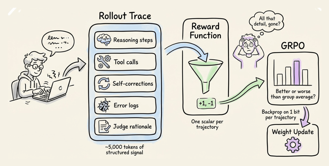
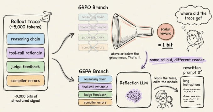
GRPO needs tens of thousands of rollouts to converge. Each rollout produces a 5,000-token trace full of reasoning steps, tool calls, and self-corrections, but GRPO reduces all of it to a single scalar reward.
So we end up backpropagating on one bit per trajectory while throwing away thousands of bits of structured signal.
GEPA takes a different approach.
Instead of computing policy gradients on that scalar, it hands the full rollout trace to a reflection LLM and asks “what went wrong, and how should the prompt change?”
The reflection model writes a new prompt, you test it, and if it improves, you keep it.
The paper came out in July 2025. It was accepted at ICLR 2026, DSPy made it a first-class optimizer, and Hugging Face and OpenAI both shipped cookbooks around it.
On compound AI systems (multi-module pipelines with separate prompts), GEPA matches or beats GRPO while spending 10-50x less compute and requiring no training infrastructure at all.
Let’s break down why it works, how it compares to GRPO, and how to use it in DSPy.
We started a course series on RL recently. Read Part 1 here →
This first chapter covers:
what makes RL fundamentally different from supervised and unsupervised learning
the agent-environment interaction loop
the exploration-exploitation tradeoff
multi-armed bandits as the simplest RL setting, four action-selection strategies (greedy, ε-greedy, optimistic initialization, UCB)
and a complete hands-on implementation of the classic 10-armed testbed with results and analysis.
The signal compression problem in RL
Reinforcement learning on language models has a signal problem that most practitioners overlook. Every rollout an agent produces is a 5,000-token document, containing:
Reasoning steps
Tool calls
Self-corrections
Compiler errors
Judge rationales
That trace is rich and structured, containing exactly the kind of diagnostic information you’d want to learn from.
While training the agent, GRPO takes all of that and reduces it to a single number.
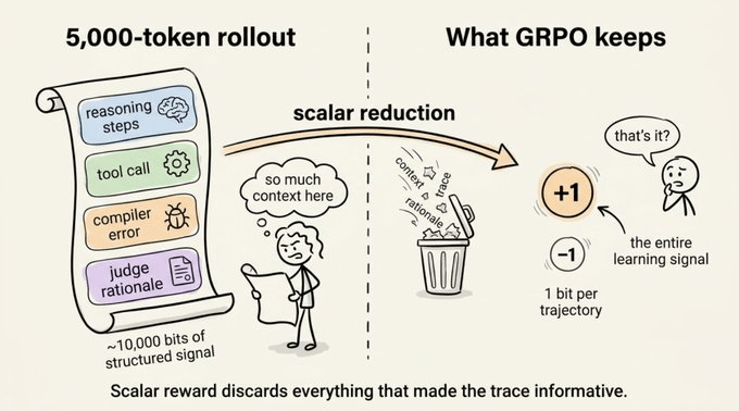
And it throws away thousands of bits of structured info, which partly explains why it needs tens of thousands of rollouts to converge.
The signal isn’t sparse, but the final reward makes it sparse.
Letting the signal read itself
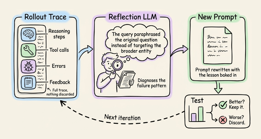
GEPA’s core idea is that the rollout is already a natural language artifact, so let an LLM read it. Don’t reduce the trace to a number.
Hand it to a reflection model along with the failure mode, and ask: “What went wrong here, and how should the prompt change?”
The reflection model writes a new prompt. You test it. And if it improves, you keep it.
That’s the full optimization loop. Everything else in the paper is engineering that makes it work at scale.
What GEPA actually optimizes
GEPA targets compound AI systems.
A pipeline of LLM modules with their own prompts, glued together by Python control flow. For instance, a multi-hop QA agent might have:
A first-hop query writer
A retriever
A summarizer
A second-hop query writer
A final answerer
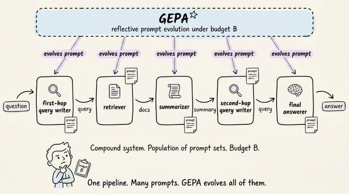
Each module has a prompt. GEPA evolves all of them.
The optimization target is simple: maximize expected metric on your task, subject to a rollout budget. The novelty is in how you spend that budget.
The feedback function
GEPA replaces your scalar metric with a feedback function μ_f.
It includes the same score that GRPO gives plus a natural language description of what happened.
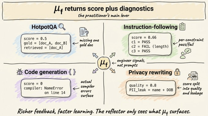
For multi-hop QA, it returns which gold docs you retrieved and which you still need.
For instruction-following, it returns per-constraint pass/fail descriptions.
For code generation, it returns the actual compiler errors and profiler traces.
For privacy-preserving rewriting, it splits the score into quality and PII-leakage with breakdowns.
The 6-step algorithm
Each iteration of the main loop does this:
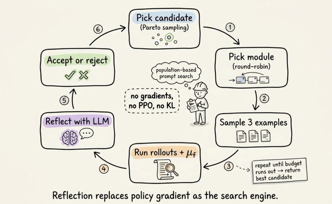
Pick a candidate prompt set from the population (Pareto sampling, more on this below)
Pick a module to mutate (round-robin across modules)
Sample 3 examples from the training set
Run rollouts and collect full traces plus feedback from μ_f
Reflect: feed traces and feedback to a reflection LLM, get a new prompt
Accept or reject: rerun on the same 3 examples. If better, keep it. If not, discard.
Repeat until the budget runs out and return the best candidate. The entire loop runs without gradients, PPO, or KL penalties.
GEPA vs GRPO, head to head
A quick look at GRPO first:
Both GRPO and GEPA take feedback and improve the system. That’s where the similarity ends.
GRPO updates model weights with policy gradients on scalar rewards. GEPA updates prompts with natural language reflection on full traces.
Here’s the side-by-side comparison:
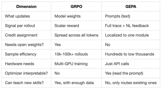
One important caveat. GRPO can change what your model knows. GEPA can only change how you ask it.
If your base model can’t do the task at all, no prompt evolution will save you. Fine-tune when you need new capabilities. Use GEPA when you need to extract more from what’s already there.
A real example
Let’s make this concrete with a real example from the paper.
The task: HotpotQA is a multi-hop question answering benchmark. You get a question that needs information from two different Wikipedia articles to answer. You can’t find the answer in just one place.
Example question: “What is the population of the region containing the parish of São Vicente?”
To answer this, your agent has to:
1st hop → Search “São Vicente parish”, retrieve a doc, learn it’s in Madeira.
2nd hop → Search “Madeira population”, retrieve that doc, get the number.
Answer: Combine both
The agent has separate modules for each hop. We’re going to look at the prompt for the second-hop query writer, the module that decides what to search for after the first retrieval.
Inputs the module receives:
question: the original user question
summary_1: a summary of what the first hop retrieved
Output it produces:
query: the search query for the second hop
Here’s the seed prompt that DSPy gives you by default:
“Given the fields question, summary_1, produce the fields query.”
This is generic since it just describes the schema and it scores around 38% on validation.
GEPA runs this on a few examples and watches what happens. For instance, the query writer might keep doing the same thing wrong, like it paraphrases the original question and retrieves the same documents it already had.
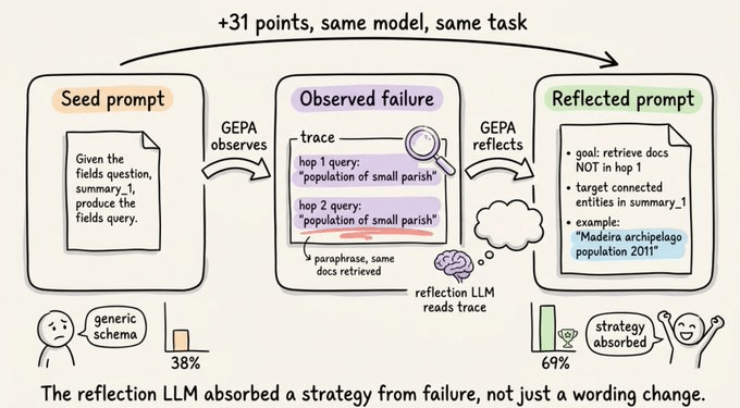
For our São Vicente example, given a summary about the parish, it would search “São Vicente parish population” again, retrieve nothing new and fail.
The reflection LLM sees this failure pattern across multiple examples in the trace. It writes a new prompt:
“Generate a search query optimized for the second hop of multi-hop retrieval. The first-hop query was the original question, so first-hop docs already cover the entities mentioned directly. Your goal: retrieve documents NOT found in the first hop but necessary to answer completely. Avoid paraphrasing the original question. Target connected or higher-level entities mentioned in summary_1 but not explicitly in the question. Example: if summary_1 describes a parish but the question asks about the wider region’s total population, your query should target the region, not the parish. So for a question about São Vicente’s region, query ‘Madeira archipelago population’ rather than ‘São Vicente population’.”
That rewritten prompt scores 69%, up from 38% on the seed.
The model and task stayed identical. The only thing that changed was the prompt for one module out of several.
The reflection LLM didn’t just rephrase the seed but it also absorbed an actual strategy from observed failures:
Don’t paraphrase the question
The first hop already covered the directly-mentioned entities
Target the broader entity that connects them
Here’s a worked example of the pattern
That’s the kind of information you cannot encode in a policy gradient. RL would just tell you “this trajectory was 0.3 below the group mean” and let backprop figure it out across thousands of tokens. GEPA writes the lesson down in plain English and ships it as the new prompt.
Pareto selection
The idea of evolving/optimizing the prompt is not new.
But most approaches often mutate from the best candidate so far, which sounds reasonable, but it collapses to local optima fast.
GEPA uses something smarter, borrowed from quality-diversity optimization.
Imagine three candidate prompts and four tasks:
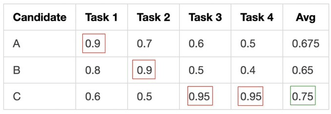
A greedy approach will pick C every time since it has the best average.
But A is the only one who handles Task 1 well, and B does Task 2 well. If you only mutate C, you lose those strategies forever.
Pareto selection keeps anyone who’s best at at least one task. Then it samples parents weighted by how many tasks they win. So C is most likely to be picked, but A and B stay in the pool. Their distinctive strengths can later be combined with C’s.
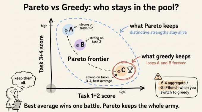
This single design choice is what separates GEPA from earlier evolutionary prompt methods.
Where GEPA fits in the landscape
Quick map of who does what:
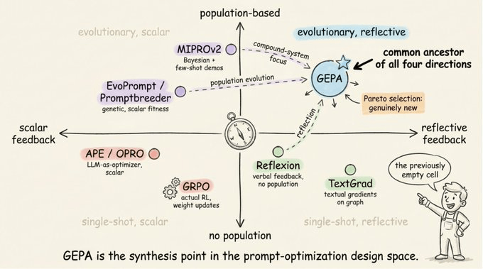
APE, OPRO: Both use an LLM to propose prompt candidates scored by a scalar metric. APE generates candidates from input-output demos and picks the best. OPRO feeds prior prompts and their scores into a meta-prompt so the LLM can propose informed improvements. Single prompt, no reflection on traces.
EvoPrompt, Promptbreeder: Evolutionary operators (crossover, mutation) applied to prompt populations via LLM calls. Promptbreeder adds a self-referential layer: it also evolves the mutation-prompts themselves. Both use scalar fitness for selection and target single prompts, not multi-module pipelines.
Reflexion: Agents reflect on task feedback after each trial and store reflections in an episodic memory buffer for the next attempt. Improves per-instance behavior across retries, not population-level prompt evolution across a training set.
TextGrad: PyTorch-style backpropagation but with natural language critiques instead of numerical gradients. An LLM propagates textual feedback through a computation graph to produce per-variable improvement suggestions. Single candidate per iteration, no population.
MIPROv2: DSPy’s prior flagship. Bootstraps few-shot examples from training data, proposes instruction candidates grounded in data summaries and traces, then uses Bayesian Optimization (Optuna TPE) to search the joint instruction-demo space across all modules. Generates all candidates upfront rather than evolving them through reflection.
GRPO: Actual RL with weight updates. Samples a group of rollouts per prompt, uses the group mean as baseline to compute per-trajectory advantage, then updates weights via policy gradients with a KL penalty. The only method here that changes what the model knows, not just how you prompt it.
GEPA borrows ideas from several of these methods. It uses verbal reflection like Reflexion, but applies it across a population of candidates instead of a single agent’s memory.
It evolves that population using selection pressure like EvoPrompt, but with natural language feedback driving mutations instead of scalar fitness.
It targets compound multi-module pipelines like MIPROv2, but evolves prompts iteratively through reflection instead of generating all candidates upfront.
The piece that’s new to GEPA is Pareto selection, which preserves candidates that are best at even one task rather than always mutating from the highest-average performer.
Using it in DSPy
The API is one line different from MIPROv2:
optimizer = dspy.GEPA(
    metric=metric_with_feedback,
    auto="medium",
    reflection_minibatch_size=3,
    candidate_selection_strategy="pareto",
    reflection_lm=dspy.LM("gpt-5", temperature=1.0, max_tokens=32000),
    use_merge=True,
    track_stats=True,
)

optimized = optimizer.compile(program, trainset=train, valset=val)
The catch: your metric function needs the right signature.
def metric(gold, pred, trace=None, pred_name=None, pred_trace=None):
    # return dspy.Prediction(score=float, feedback=str)
Return a prediction with both a score and a feedback string. The feedback is what gets fed to the reflection LLM, so make it diagnostic and specific.
If your feedback string is just “wrong answer”, you’re back to scalar territory, and GEPA degrades to a slower MIPROv2.
If your feedback says “missed entity X, retrieved doc Y when gold was Z, format violation in step 3”, then GEPA works well with that level of detail.
A 2026 reality check
GEPA beats GRPO specifically, not every RL method.
The field has stopped framing this as GEPA vs RL and started framing it as GEPA and RL. The paper itself points to hybrid recipes as the natural next step.
Reflection is far more sample-efficient than RL on compound systems. The two are increasingly combined, not pitted against each other.
One more nuance worth knowing is that Decagon’s March 2026 production ablations found that more data isn’t always better with GEPA. 20 to 100 examples often beats 500. The reflection loop overfits when you feed it too much.
GEPA learns from patterns in failures. With 50 well-chosen examples, the reflector sees a clean signal. With 500, it starts chasing noise.
Use small, high-quality training sets and don’t assume scale helps.
When to reach for what
If you’re building a compound AI system today, here’s the decision tree.
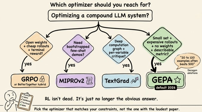
Use GEPA when: You have a small training set, expensive rollouts, no access to weights, and a metric you can describe in words.
Use GRPO when: You have abundant cheap rollouts, open weights, and a verifiable terminal reward.
Use MIPROv2 when: You specifically need bootstrapped few-shot exemplars in your prompts.
Use TextGrad when: Your computation graph is deep and you want explicit per-variable critique propagation.
For most practical compound-system work in 2026, GEPA is the default to try first.
RL still has its place, but it’s no longer the obvious default when reading a rollout costs less than running ten thousand more.
To dive deeper into RL, we started a course series on RL recently. Read Part 1 here →
The first chapter covers:
what makes RL fundamentally different from supervised and unsupervised learning
the agent-environment interaction loop
the exploration-exploitation tradeoff
multi-armed bandits as the simplest RL setting, four action-selection strategies (greedy, ε-greedy, optimistic initialization, UCB)
and a complete hands-on implementation of the classic 10-armed testbed with results and analysis.
Thanks for reading!