

Loading an LLM is only the first part of GPU memory planning.
Model weights stay roughly fixed during inference. The KV cache does not. It grows with every token in the sequence, and by default, every active sequence needs its own cache.
For Llama 3.1 70B, one 128K-token sequence requires about 40 GB of BF16 KV cache. Four full-length sequences would add another 160 GB, before accounting for model weights and serving overhead.
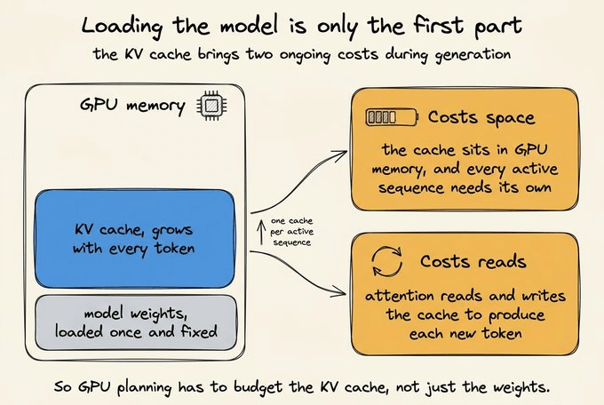
That creates two separate costs. The cache occupies GPU memory, and the attention layers must repeatedly read it while generating new tokens.
The techniques described as KV cache optimizations address different parts of this problem. Some change what the model stores. Some retain fewer tokens or use fewer bits. Others leave the logical cache intact and improve how the serving engine reads, allocates, shares, or moves it.
This article organizes twelve techniques by what they reduce, when they can be applied, and what trade-off remains. Each section includes a small runnable example that explains the main idea.
To dive deeper into the full LLMOps lifecycle, we have covered every bit of this in the LLMOps course, starting from fundamentals to production.
The cache formula
Each attention layer stores one key and one value for every retained token.
The raw cache size for one sequence is:
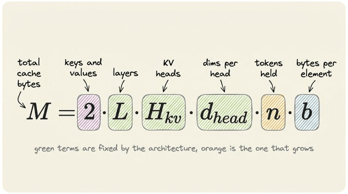
The leading 2 counts keys and values. BF16 uses two bytes per value, while FP8 uses one.
That formula also gives us a clean way to group the techniques:
GQA and MQA reduce the number of KV heads.
Cross-layer attention reduces the number of unique cached layers.
Sliding windows and eviction reduce the number of retained tokens.
MLA reduces the width of the stored representation.
Quantization reduces the bytes used by each value.
Hybrid recurrent layers replace a growing cache with fixed-size state.
Paging and prefix reuse reduce allocation waste and duplicate blocks.
Sparse attention needs a separate line. It may read fewer tokens without removing them from memory, so it can cut attention work while leaving cache capacity unchanged.
This distinction matters when the GPU is full. A faster attention kernel doesn’t create room for another sequence unless it also stores fewer bytes.
Technique map
The visual below puts all 12 techniques in one place, showing what each one changes and whether its main saving comes from fewer heads, layers, tokens, dimensions, bits, or duplicated memory.
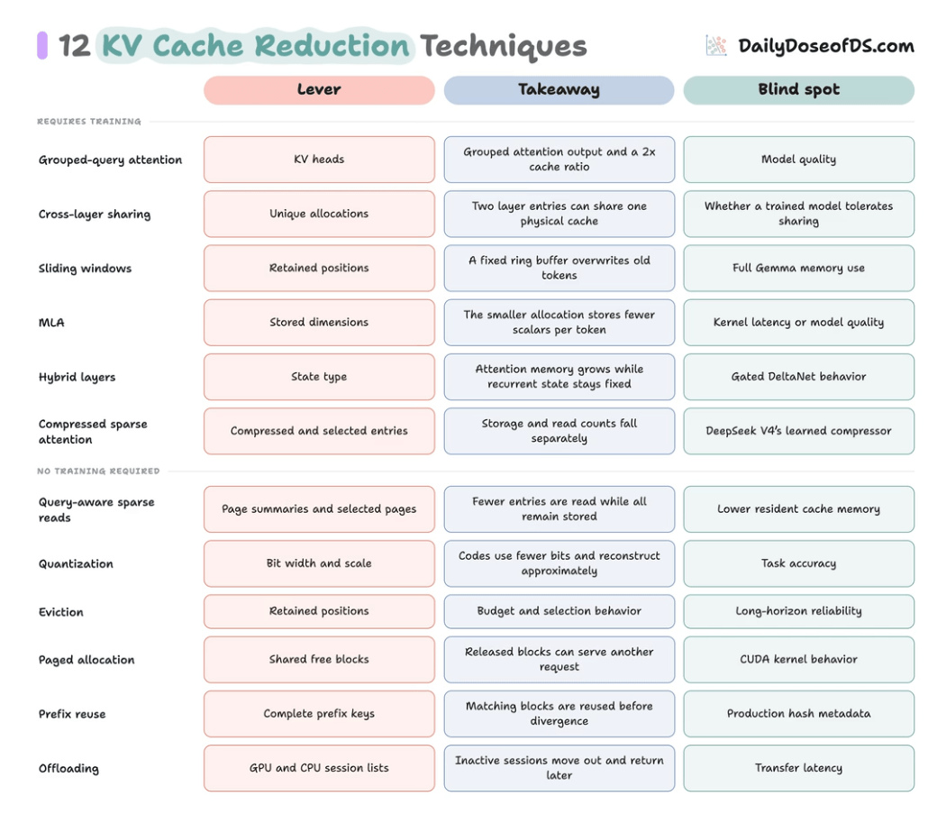
The table above represents what each technique tries to tackle.
The rest of the article works through the full table in order.
1. GQA and MQA cache fewer heads
The cache formula above contains a term for KV heads. Reducing that term is one of the largest architectural savings available.
Inside each transformer layer, every token produces three representations:
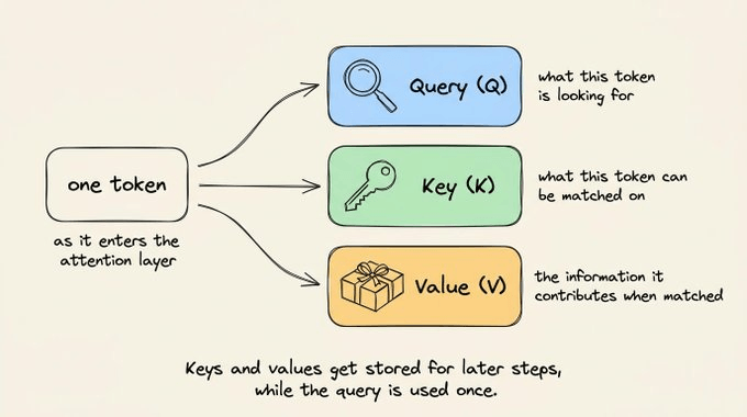
The query represents what the current token needs.
The key describes what each earlier token can match.
The value carries the information returned when that match receives attention.
During generation, the current token’s query is compared with cached keys.
Those comparisons produce attention weights, which combine the cached values. The layer keeps keys and values for later decoding steps. It does not keep the queries.
Attention splits these representations into smaller parts called heads.
A query head is one slice of the token’s query representation. It is not the user’s prompt or a separate model request. Different heads can learn to focus on different relationships in the same sequence.
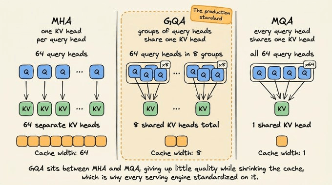
Standard multi-head attention, or MHA, gives each query head a matching key head and value head. A layer with eight query heads therefore produces eight key heads and eight value heads. Every attention layer performs this projection independently and keeps its own KV cache.
Multi-query attention, or MQA, keeps all eight query heads but produces only one key head and one value head. Every query head reads from that shared KV pair. The sharing does not cross transformer layers.
Grouped-query attention, or GQA, sits between these two layouts. It divides the query heads into groups and assigns one KV pair to each group. With eight query heads and two KV heads, four query heads share each KV pair.
All three methods operate inside each attention layer. They differ only in how many KV heads that layer stores. Cross-layer attention, covered next, is a separate idea that shares cached information between layers.
The GQA paper described it as an intermediate point between MHA and MQA.
The authors converted existing MHA checkpoints and used 5 percent of the original pretraining compute for recovery training. Their uptrained GQA models stayed close to MHA quality while approaching MQA speed.
The following example uses eight query heads. It shows which KV head each query head reads. It also counts the cached scalars for six tokens:
query_heads = 8
tokens = 6
head_size = 8

for name, kv_heads in [("MHA", 8), ("GQA", 2), ("MQA", 1)]:
    queries_per_kv_head = query_heads // kv_heads
    mapping = [head // queries_per_kv_head for head in range(query_heads)]
    cached_scalars = 2 * kv_heads * tokens * head_size

    print(name, "mapping:", mapping)
    print(name, "cached scalars:", cached_scalars)

# Output:
"""
MHA mapping: [0, 1, 2, 3, 4, 5, 6, 7]
MHA cached scalars: 768
GQA mapping: [0, 0, 0, 0, 1, 1, 1, 1]
GQA cached scalars: 192
MQA mapping: [0, 0, 0, 0, 0, 0, 0, 0]
MQA cached scalars: 96
"""
The mapping lists one KV head number for every query head. MHA uses a different KV head each time. GQA shares KV head 0 across four queries, then does the same with KV head 1. MQA maps every query head to KV head 0.
The cache count includes both keys and values. It then multiplies by six tokens and eight scalars per head.
Llama 3.1 70B uses 64 query heads and 8 KV heads. At 128K context, that produces a 40 GB BF16 cache instead of the 320 GB required by the same shape with 64 KV heads.
This code proves the storage ratio. It doesn’t test quality, because head sharing changes what the model learns and must be evaluated after training.
2. Cross-layer attention
GQA shares keys and values across heads within one layer. Cross-layer attention shares them across adjacent layers.
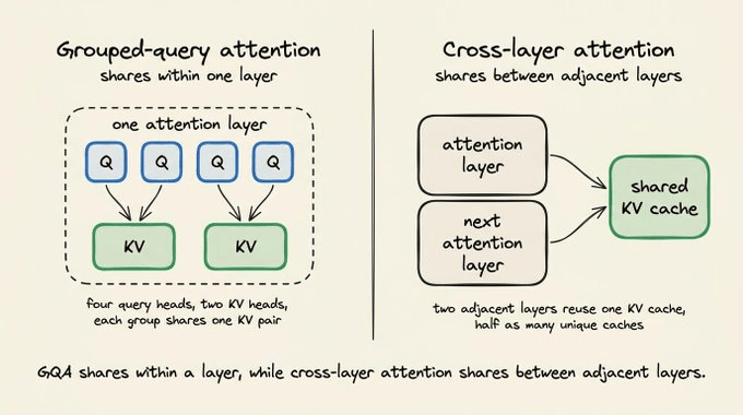
So a sharing factor of two implies two attention layers use one set of cached keys and values. The model now stores half as many unique layer caches.
The Cross-Layer Attention (CLA) paper trained 1B and 3B models and reported another 2x KV cache reduction while keeping accuracy close to the MQA baseline.
The next script represents two layers sharing one cache allocation:
tokens = 32
kv_heads = 2
head_size = 8

one_layer_cache = 2 * tokens * kv_heads * head_size
shared_cache = {"stored_scalars": one_layer_cache}
layer_caches = [shared_cache, shared_cache]

separate_total = 2 * one_layer_cache
shared_total = shared_cache["stored_scalars"]

print("layers point to same cache:", layer_caches[0] is layer_caches[1])
print("two separate layer caches:", separate_total, "scalars")
print("one shared layer cache:", shared_total, "scalars")

# Output:
"""
layers point to same cache: True
two separate layer caches: 2048 scalars
one shared layer cache: 1024 scalars
"""
One layer would store 1,024 scalars here. The leading 2 counts keys and values. Two independent layers would therefore store 2,048 scalars.
Both items in layer_caches point to the same Python object. The physical storage remains 1,024 scalars even though two logical layers use it.
Cross-layer sharing compounds GQA because it reduces a different term. GQA stores fewer KV heads inside each layer. CLA stores fewer distinct layer caches across the model.
A standard checkpoint learns separate KV projections for every layer. Each layer expects the cache created by its own weights. Redirecting it to another layer’s cache changes the model’s computation.
A CLA model trains with the sharing pattern already present. Training lets each dependent layer adapt to the shared cache. The serving engine must then reproduce the same ownership pattern.
The checkpoint and engine must agree on which layer owns each cache. This is why CLA cannot be enabled as a generic runtime flag.
3. Sliding windows
CLA reduces the number of stored layer caches. Sliding-window attention reduces the tokens stored inside selected layers.
In full self-attention, each new token can attend to every earlier token. Each attention layer must therefore keep keys and values for the full sequence. As the sequence grows, every layer’s KV cache grows with it.
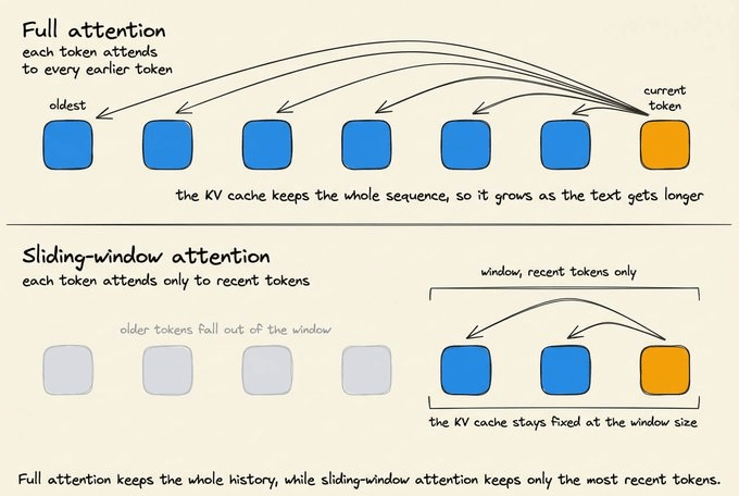
Sliding-window attention limits a layer to recent tokens. Suppose the window contains 1,024 positions. That layer stores KV entries for only the latest 1,024 tokens. Each new entry removes the oldest one after the window fills. Its cache then stays fixed at 1,024 positions.
We call this a local layer because it sees nearby context. A global layer can still attend to every earlier token. Its cache keeps growing until the sequence ends.
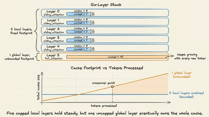
Many models mix both layer types. Local layers provide most of the memory saving. Occasional global layers preserve access to distant parts of the prompt. The total cache still grows, but much slower than full attention everywhere.
For instance, Gemma 3 uses a repeating pattern of five local layers followed by one global layer. Its local window is 1,024 tokens, while the global layer supports the full 128K context:
The following example tracks the positions retained by a four-token window:
window_size = 4
retained_positions = []

for position in range(10):
    retained_positions.append(position)

    if len(retained_positions) > window_size:
        retained_positions.pop(0)

    print(f"after token {position}: {retained_positions}")

print("maximum retained positions:", window_size)

# Output:
"""
after token 0: [0]
after token 1: [0, 1]
after token 2: [0, 1, 2]
after token 3: [0, 1, 2, 3]
after token 4: [1, 2, 3, 4]
after token 5: [2, 3, 4, 5]
after token 6: [3, 4, 5, 6]
after token 7: [4, 5, 6, 7]
after token 8: [5, 6, 7, 8]
after token 9: [6, 7, 8, 9]
maximum retained positions: 4
"""
The list fills with positions 0 through 3. When position 4 arrives, the list becomes too long. Removing its first item drops position 0.
The same step repeats for every later token. Production engines usually use a ring buffer, which overwrites old slots without moving the remaining entries.
The first four tokens fill the available slots. Token 4 then removes token 0, so the window shifts to positions 1 through 4. Every later token shifts that range forward by one. After token 9, only positions 6 through 9 remain. The allocation stays fixed at four slots throughout.
The ratio also changes with context length. Below 1,024 tokens, both layouts retain the same number of positions. The saving appears only after the sequence exceeds the local window.
4. Multi-head latent attention
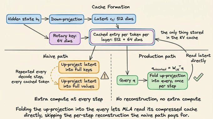
Multi-head latent attention, or MLA, doesn’t cache a complete key and value for every head. It compresses the hidden state into a smaller latent representation and stores that instead.
During decode, the model uses learned projections to recover the information needed by attention.
Implementations can absorb parts of those projections into the query and output paths, which avoids reconstructing every full KV tensor in memory.
DeepSeek-V2 introduced this design. The paper reported a 93.3 percent KV cache reduction compared with DeepSeek 67B and a 5.76x increase in maximum generation throughput:
An actual MLA layer uses learned matrices to create and use the latent representation. Those matrix operations hide the basic memory difference in a small example.
The following example counts storage for one token. The dimensions are intentionally small. They make the difference between both layouts visible.
kv_heads = 4
head_size = 8

standard_keys = kv_heads * head_size
standard_values = kv_heads * head_size
standard_total = standard_keys + standard_values

mla_latent = 8
mla_rotary_key = 4
mla_total = mla_latent + mla_rotary_key

print("standard cache:", standard_keys, "key +", standard_values, "value")
print("MLA cache:", mla_latent, "latent +", mla_rotary_key, "rotary key")
print("stored scalars per token:", standard_total, "->", mla_total)
print(f"example reduction: {standard_total / mla_total:.2f}x")

# Output:
"""
standard cache: 32 key + 32 value
MLA cache: 8 latent + 4 rotary key
stored scalars per token: 64 -> 12
example reduction: 5.33x
"""
Four KV heads with eight scalars each produce 32 key scalars. The values require another 32. Standard attention therefore stores 64 scalars per token.
The illustrative MLA layout stores eight latent scalars and four positional scalars. Its total is 12. Dividing 64 by 12 gives the example ratio.
The 5.33x figure belongs only to this example. Real MLA models choose different latent and positional dimensions.
MLA is not an inference flag for a standard checkpoint. Its projection weights and cache layout belong to the trained model. Converting another model still requires training.
5. Replace growing cache with fixed state using Hybrid models
Mamba and recurrent linear-attention layers don’t store one key and value for every old token. They update a fixed-size state as the sequence grows.
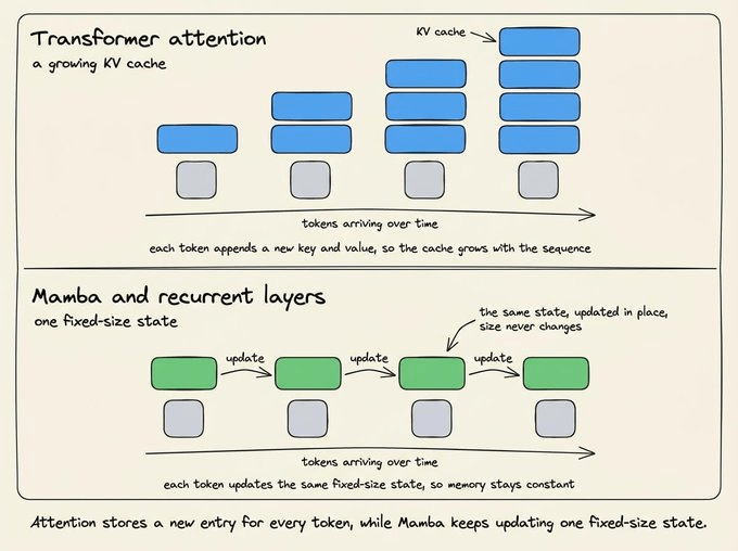
Pure recurrent models keep memory nearly constant with context, but full attention remains better at exact retrieval in many settings. Recent models combine both.
Qwen3-Next has 48 layers arranged as 12 repeated blocks. Each block contains three Gated DeltaNet layers and one full-attention layer. Only the 12 full-attention layers create a standard growing KV cache.
The model card reports 16 query heads, 2 KV heads, and a head dimension of 256 for those attention layers.
The next example compares their memory growth. The attention layer stores one 64-value key and value per token. The recurrent layer keeps one fixed 64-by-64 state.
width = 64
bytes_per_value = 4

attention_values_per_token = 2 * width
recurrent_state_values = width * width

for tokens in [128, 4096]:
    attention_kb = tokens * attention_values_per_token * bytes_per_value // 1024
    recurrent_kb = recurrent_state_values * bytes_per_value // 1024

    print(f"{tokens} tokens")
    print("  attention KV:", attention_kb, "KB")
    print("  recurrent state:", recurrent_kb, "KB")

# Output:
"""
128 tokens
  attention KV: 64 KB
  recurrent state: 16 KB
4096 tokens
  attention KV: 2048 KB
  recurrent state: 16 KB
"""
The attention calculation multiplies storage per token by sequence length. The recurrent calculation does not use tokens at all. Its state remains the same size in both cases.
The example tracks memory only. It does not implement Mamba or Gated DeltaNet. Those architectures use learned update rules to decide what the fixed state retains.
The attention cache grows 32x between the two sequence lengths. The recurrent state remains 16 KB. Hybrid models pay linear cache growth only in their full-attention layers.
For the Qwen3-Next attention shape, 12 full-attention layers require 3 GB of BF16 KV at 128K context.
Making all 48 layers full attention would raise that growing portion to 12 GB.
Jamba shows the same design choice with a different ratio. It interleaves one attention layer with seven Mamba layers. At 256K context, the Jamba paper reports a 4 GB KV cache, compared with 32 GB for Mixtral.
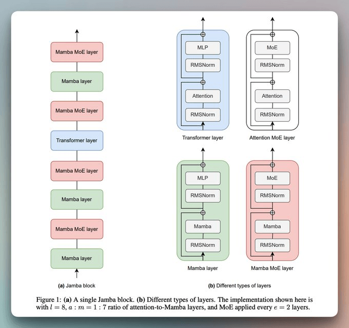
This layout belongs to the trained model. A serving engine cannot replace arbitrary attention layers with recurrent ones at runtime.
6. Compressed sparse attention
Full attention does two expensive things. It stores a separate KV entry for every earlier token, then reads every stored entry when generating the next token.
Sparse attention changes only the second part.
It reads fewer entries for each new token, but it may still keep the complete cache in memory. That can make generation faster without making the resident KV cache smaller.
Compressed sparse attention focuses on optimizing both parts.
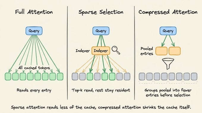
First, it combines several neighbouring token entries into one compressed entry. It stores that shorter sequence instead of one long-range entry per token.
Then, for each new token, a selector chooses only the compressed entries that appear most relevant. Attention reads that selected subset.
DeepSeek V4 uses this design.
If the compression factor is m, every m token entries become one stored entry. So a context of n tokens produces roughly n / m compressed entries.
The model then selects k of those entries for attention. A small sliding window preserves finer detail for the most recent tokens.
At one million tokens, DeepSeek reports that V4-Pro uses 10 percent of the KV cache and 27 percent of the single-token inference FLOPs required by DeepSeek V3.2. V4-Flash goes further at 7 percent of the cache and 10 percent of the FLOPs
These are whole-model results. They include V4’s hybrid attention layout and precision choices, so they should not be read as the isolated effect of compression alone.
The next block isolates the two reductions. Compressing 32 long-range entries in groups of four leaves eight stored entries. If attention selects two of those eight, it reads only two compressed entries for the current step.
full_token_entries = 32
tokens_per_group = 4
selected_entries = 2

compressed_entries = full_token_entries // tokens_per_group

print("full token entries:", full_token_entries)
print("compressed entries stored:", compressed_entries)
print("compressed entries read:", selected_entries)
print("storage reduction:", f"{full_token_entries / compressed_entries:.0f}x")

# Output:
"""
full token entries: 32
compressed entries stored: 8
compressed entries read: 2
storage reduction: 4x
"""
Dividing 32 tokens into groups of four creates eight compressed entries. That is the storage reduction. Selecting two of those eight entries is the separate attention-work reduction.
The cache now holds eight long-range entries instead of 32. Attention reads two of them. A small local window separately preserves recent token detail.
This technique has to be built into the model and training process. A serving engine cannot convert an existing full-attention model into compressed sparse attention by changing a cache setting.
7. Query-aware sparse reads
The previous technique reduced both storage and attention work.
Sometimes, changing the model architecture is not an option. We may still want to reduce how much cache each decode step reads.
Recall what happens while the model generates a token. The new token produces a query, which acts like a search signal. Full attention compares it with every stored key. A long prompt therefore forces the GPU to load a large cache repeatedly.
Quest is a technique that reduces those reads without deleting any KV entries.
It divides the cache into pages.
A page is a small group of neighbouring token entries.
Each page also stores the minimum and maximum key values found inside it.
For every new query, Quest scores these short page summaries first. It then loads only the pages with the highest scores. The full cache remains stored because a page ignored now may matter later.
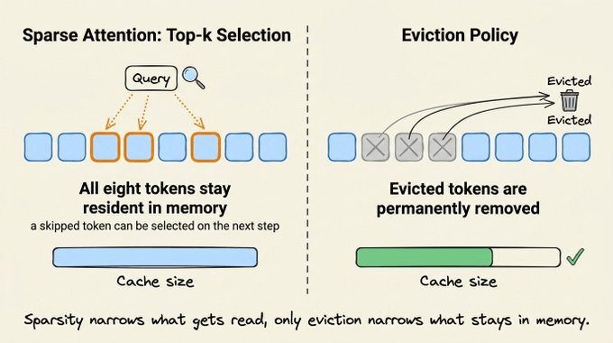
The Quest paper reports up to 7.03x lower self-attention latency. Its complete inference system reached up to 2.23x speedup.
The example below uses four pages. Each page contains two keys. A key has only two numbers here, which keeps the scoring visible.
import numpy as np

pages = np.array([
    [[1, 0], [2, 1]],
    [[5, 1], [4, 2]],
    [[0, 6], [1, 5]],
    [[-2, -1], [-1, 0]],
])
query = np.array([1.0, 0.5])

page_min = pages.min(axis=1)
page_max = pages.max(axis=1)
page_scores = np.maximum(query * page_min, query * page_max).sum(axis=1)
selected_pages = np.argsort(page_scores)[-2:]

for page, score in enumerate(page_scores):
    print(f"page {page} score: {score:.1f}")

print("selected pages:", np.sort(selected_pages).tolist())
print("KV entries read:", len(selected_pages) * 2, "of", pages.size // 2)
print("KV entries still stored:", pages.size // 2)

# Output:
"""
page 0 score: 2.5
page 1 score: 6.0
page 2 score: 4.0
page 3 score: -1.0
selected pages: [1, 2]
KV entries read: 4 of 8
KV entries still stored: 8
"""
The pages array contains eight keys in total. The next two lines create one minimum and one maximum summary per page. Quest uses similar summaries to estimate a page’s best possible attention score.
The query prefers large values in both key dimensions. Pages 1 and 2 receive the highest scores, so the example reads their four keys. It leaves the other four keys untouched during this step.
If you notice the last line, the step reads four entries, but all eight remain resident. Quest reduces cache traffic and attention work. It does not reduce the memory needed to hold the full cache.
In practice, Quest uses many-dimensional keys and dedicated GPU code. It also repeats the selection for every query.
8. Quantization
Quest keeps every KV entry and skips some reads. Quantization takes another route. It keeps every entry but stores each number with fewer bits.
Keys and values normally contain floating-point numbers. BF16 stores each number with 16 bits. FP8 uses 8 bits, so its raw payload is roughly half as large. A 4-bit format cuts the payload to 25%.
Quantization maps many original numbers onto a smaller set of allowed values. A scale controls the gap between those values. The engine stores the small integer code and enough scale information to interpret it later.
The choice of scale affects accuracy. One extreme value can make a shared scale too wide. Most ordinary values then get rounded too aggressively.
KIVI handles keys and values differently. It groups key values by channel, which means the same feature across tokens. It groups value-cache numbers by token. The KIVI paper reports 2.6x lower peak memory and up to 4x larger batches with its 2-bit cache.
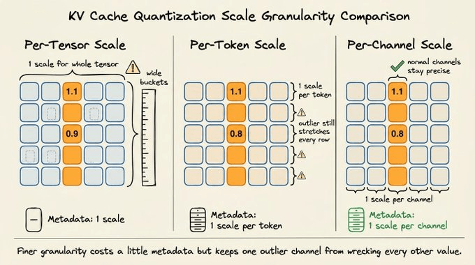
The small example below shows the basic mapping. It converts six BF16-style values into signed 4-bit codes. It then converts those codes back into approximate values.
import numpy as np

values = np.array([-1.0, -0.55, -0.10, 0.25, 0.60, 1.0])
bits = 4
largest_code = 2 ** (bits - 1) - 1
scale = np.max(np.abs(values)) / largest_code

codes = np.rint(values / scale)
codes = np.clip(codes, -largest_code, largest_code).astype(np.int8)
restored = codes * scale

print("original values:", values.tolist())
print("4-bit codes:", codes.tolist())
print("restored values:", np.round(restored, 3).tolist())
print("raw payload:", len(values) * 16, "bits ->", len(values) * 4, "bits")

# Output:
"""
original values: [-1.0, -0.55, -0.1, 0.25, 0.6, 1.0]
4-bit codes: [-7, -4, -1, 2, 4, 7]
restored values: [-1.0, -0.571, -0.143, 0.286, 0.571, 1.0]
raw payload: 96 bits -> 24 bits
"""
Signed 4-bit storage provides codes from -7 through 7 in this example. Dividing by scale maps each original value to a code. Multiplying by the same scale produces the approximate value used during attention.
As you may have noticed, the restored values are close, but not identical. That rounding difference is quantization error. The final line counts only the six stored values. A real cache also stores scale metadata.
The example uses one scale for all six values. KIVI uses smaller groups because each group can fit its own numerical range. This usually reduces rounding error, though it requires more scale metadata.
If you use vLLM, it exposes FP8 cache storage directly:
MODEL_ID=Qwen/Qwen2.5-7B-Instruct
vllm serve "$MODEL_ID" --kv-cache-dtype fp8
The first line defines the model name. The second starts a vLLM server and asks it to store the KV cache in FP8. This command keeps running because it launches the inference server.
Recent vLLM versions can also leave selected layers in their native type. This is useful when a sliding-window layer proves more sensitive:
MODEL_ID=google/gemma-3-4b-it
vllm serve "$MODEL_ID" \
  --kv-cache-dtype fp8 \
  --kv-cache-dtype-skip-layers sliding_window
This version leaves sliding-window layers in their original format. It quantizes the remaining cache layers. The option helps when those local-attention layers lose too much accuracy under FP8.
Quantization preserves every token position. The next technique reduces memory by removing positions instead.
9. Eviction
Quantization keeps all token positions. That may still be too large for a long context. Eviction sets a fixed position budget and discards entries outside it.
The difficult question is which positions should not be evicted. Recent tokens often matter because they contain the current conversation. Older tokens may still carry instructions, facts, or tool results needed later.
H2O is a technique that keeps recent positions and older heavy hitters. A heavy hitter is a token that has accumulated high attention during earlier steps. Once H2O evicts another token, its KV entry is no longer available.
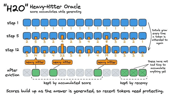
Other methods estimate importance differently. SnapKV studies attention near the end of the input prompt. It uses that observation window to choose prompt positions before generation.
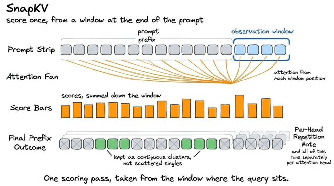
PyramidKV gives lower layers larger budgets and higher layers smaller ones, based on the attention patterns reported by its authors.
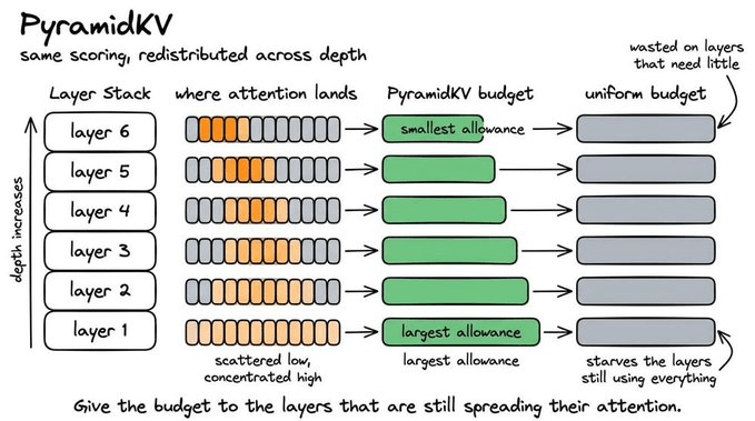
SnapKV reports 8.2x higher memory efficiency and 3.6x faster generation with 16K-token inputs. PyramidKV reports matching full-cache performance while retaining 12 percent of the cache in its LongBench experiments.
The following example takes a snapshot after ten tokens. Their scores represent attention accumulated during earlier decode steps. The cache can retain only six positions, including the latest two.
scores = [9.0, 0.2, 4.0, 0.1, 0.3, 6.0, 0.2, 0.4, 0.1, 0.2]
budget = 6
recent_count = 2

positions = list(range(len(scores)))
recent = positions[-recent_count:]
older = positions[:-recent_count]

heavy_hitter_count = budget - recent_count
heavy_hitters = sorted(
    older,
    key=lambda position: scores[position],
    reverse=True,
)[:heavy_hitter_count]

retained = sorted(heavy_hitters + recent)

print("heavy hitters:", sorted(heavy_hitters))
print("recent positions:", recent)
print("retained positions:", retained)
print("cache entries:", len(retained), "of", len(scores))

# Output:
"""
heavy hitters: [0, 2, 5, 7]
recent positions: [8, 9]
retained positions: [0, 2, 5, 7, 8, 9]
cache entries: 6 of 10
"""
Positions 8 and 9 are retained because they are the newest. Four slots remain. The sort selects positions 0, 2, 5, and 7 because they have the largest scores among older tokens.
The union of those two groups produces the final six-position cache. Positions 1, 3, 4, and 6 are discarded.
Real H2O updates its heavy-hitter statistics as generation proceeds. This smaller example starts with the accumulated scores so the selection rule remains visible.
That said, eviction needs a cautious evaluation. Importance changes across turns. A tool result that receives little attention now may become necessary after several more calls. System instructions and delimiters can also be disproportionately important.
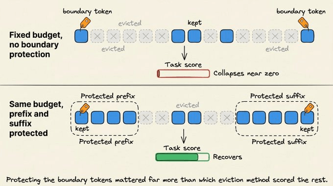
Eviction evaluations should therefore use complete agent traces and delayed references. They should also include structured prompts. A good Needle-in-a-Haystack score does not cover those cases.
10. Paging
So far, we have looked at what one request stores or reads. Paging solves a different problem: how the serving engine allocates cache memory across many requests.
A simple allocator may reserve one continuous memory region per request. It often reserves enough space for the request’s maximum length. Shorter requests leave part of that region unused. Free space also gets split into gaps as requests finish.
PagedAttention divides GPU cache memory into equal-sized blocks. Each block holds KV entries for a fixed number of tokens. A request can use blocks found anywhere in the shared pool, so its blocks do not need to lie next to each other.
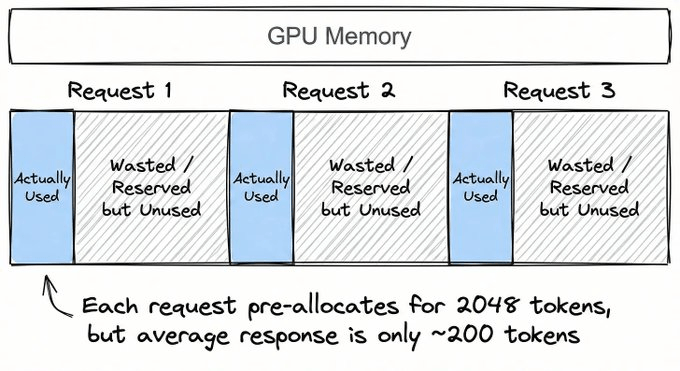
When a request finishes, the allocator returns its blocks to the pool. Another request can reuse them immediately. The PagedAttention paper reports near-zero KV cache waste and 2x to 4x higher throughput than the systems tested.
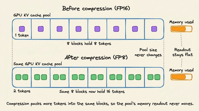
A fixed pool can hide the effect of quantization. The engine may reserve the same 8 GB before and after enabling FP8. Smaller entries increase the number of tokens that fit inside that pool. The allocated memory shown by nvidia-smi may remain unchanged.
The example below begins with six free blocks. Request A takes three. Request B takes two. A then finishes and returns its blocks before request C arrives.
free_blocks = [0, 1, 2, 3, 4, 5]

request_a = free_blocks[:3]
free_blocks = free_blocks[3:]

request_b = free_blocks[:2]
free_blocks = free_blocks[2:]

free_blocks.extend(request_a)
free_after_a = free_blocks.copy()
request_c = free_blocks[:2]
free_blocks = free_blocks[2:]

print("request A blocks:", request_a)
print("request B blocks:", request_b)
print("free after A finishes:", free_after_a)
print("request C blocks:", request_c)

# Output:
"""
request A blocks: [0, 1, 2]
request B blocks: [3, 4]
free after A finishes: [5, 0, 1, 2]
request C blocks: [5, 0]
"""
After A finishes, the free pool contains block 5 and A’s returned blocks. Request C takes blocks 5 and 0. Those block numbers are not adjacent, but the block table records their order for C.
This is the central paging idea. The allocator reuses available blocks instead of searching for one large continuous region.
vLLM also tracks which request owns each block. Its attention code can read the non-adjacent blocks in logical sequence order. The short example isolates allocation and reuse.
Quantization still changes the capacity inside this pool. An 8 GB pool holds 26,214 tokens at 320 KB per token, compared with 52,428 tokens at 160 KB. Total allocated GPU memory remains 8 GB in both cases.
11. Prefix reuse
Paging reuses blocks after a request finishes. Prefix caching can share blocks while several requests are still active. It applies when those requests begin with exactly the same tokens.
This happens often with system prompts and tool definitions. Without prefix caching, the engine computes and stores another KV copy for every request. The repeated prefix consumes memory and repeats the prefill work that created it.
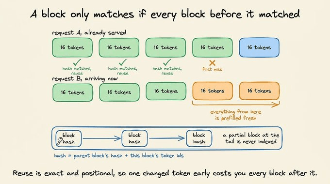
Automatic prefix caching stores each completed prefix block under a lookup key. When another request has the same token prefix, it points to the existing KV block. New computation begins only after the requests diverge.
vLLM builds each lookup key from the current block and its preceding blocks. It also includes details such as adapter identifiers when they affect compatibility. The vLLM prefix-caching design documents this structure.
The example below uses four-token blocks. Each lookup key contains the entire prefix up to that block. This is a readable stand-in for vLLM’s chained hashes.
def prefix_keys(tokens, block_size):
    block_ends = range(block_size, len(tokens) + 1, block_size)
    return [tuple(tokens[:end]) for end in block_ends]

first = [10, 11, 12, 13, 20, 21, 22, 23, 30, 31, 32, 33]
second = [10, 11, 12, 13, 20, 21, 22, 23, 40, 41, 42, 43]

cache = set()
first_keys = prefix_keys(first, block_size=4)
first_hits = sum(key in cache for key in first_keys)
cache.update(first_keys)

second_keys = prefix_keys(second, block_size=4)
second_hits = sum(key in cache for key in second_keys)

print("first request reused:", first_hits, "of", len(first_keys), "blocks")
print("second request reused:", second_hits, "of", len(second_keys), "blocks")
print("second request computes:", len(second_keys) - second_hits, "new block")

# Output:
"""
first request reused: 0 of 3 blocks
second request reused: 2 of 3 blocks
second request computes: 1 new block
"""
The first request has no cache entries to reuse. It adds keys for its first four, eight, and twelve tokens. The second request has the same first eight tokens, so its first two keys match.
The final four tokens differ. That changes the last prefix key, so the second request computes one new block.
Using the full prefix prevents a false match. Two requests cannot reuse a block merely because four tokens match somewhere in the middle. Their preceding context must match as well.
Prefix reuse depends on exact tokenized prefixes. A timestamp in the system prompt, reordered JSON keys in a tool schema, or different chat-template whitespace can break the match.
Stable prompt templates therefore improve the hit rate. The model and cache format can remain unchanged while duplicate storage drops.
12. Cache Offloading from GPU
Prefix reuse helps when another request begins with tokens the engine has already processed. Offloading handles a different problem. It moves KV blocks that are not currently needed from GPU memory to a larger but slower memory tier, usually CPU memory.
Those blocks may belong to a sequence paused by the scheduler or to a cached prefix retained for reuse. When the engine needs them again, it copies them back to the GPU.
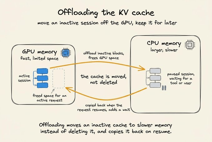
There is one important limitation. A new OpenAI-compatible API request does not automatically resume the KV cache from an earlier request. Reuse happens only if the engine still tracks the sequence, recognizes an exact prefix-cache match, or restores the cache through an external storage system.
Offloading frees GPU memory without deleting the stored KV data. It does not reduce the total number of bytes held across GPU and CPU memory. The trade-off appears when the engine must transfer those blocks back before computation can continue.
The example below gives the GPU room for two sessions. Adding session C moves the oldest session, A, to CPU memory. Resuming A brings it back and moves B out.
gpu_cache = ["cache-a", "cache-b"]
cpu_cache = []

# Cache C needs GPU space, so cache A moves to CPU memory.
cpu_cache.append(gpu_cache.pop(0))
gpu_cache.append("cache-c")

print("GPU after cache C arrives:", gpu_cache)
print("CPU after cache C arrives:", cpu_cache)

# Cache A is needed again, so it returns to the GPU.
cpu_cache.remove("cache-a")
cpu_cache.append(gpu_cache.pop(0))
gpu_cache.append("cache-a")

print("GPU after cache A returns:", gpu_cache)
print("CPU after cache A returns:", cpu_cache)

# Output:
"""
GPU after cache C arrives: ['cache-b', 'cache-c']
CPU after cache C arrives: ['cache-a']
GPU after cache A returns: ['cache-c', 'cache-a']
CPU after cache A returns: ['cache-b']
"""
The first move leaves caches B and C on the GPU while cache A remains available in CPU memory. When cache A is needed again, the example brings it back and moves cache B out.
The lists contain cache names instead of tensors. A real engine performs this operation on KV blocks and tracks which request or reusable prefix owns each block.
The example assumes that the engine has retained enough information to identify cache A later. Sending an unrelated API request with the same label would not restore it automatically.
vLLM can enable a 16 GB CPU offloading buffer directly:
MODEL_ID=Qwen/Qwen2.5-7B-Instruct

vllm serve "$MODEL_ID" \
  --kv-offloading-size 16 \
  --kv-offloading-backend native
The first option sets the CPU buffer size in GB. The second selects vLLM’s native CPU backend. Like the earlier serving command, this process keeps running after startup.
Offloading trades GPU capacity for transfer time. Measure resume latency and CPU bandwidth before enabling a large offload tier.
How to use them together
Some of these methods compose because they reduce different terms. Architecture-level methods still depend on how the checkpoint was trained.
For instance, take the 40 GB GQA cache from the first example.
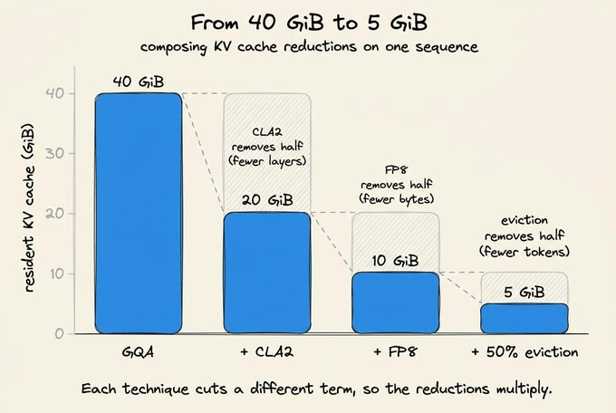
CLA2 can cut the unique layers in half, producing 20 GB.
FP8 can halve the bytes per value, producing roughly 10 GB.
A 50 percent token budget would reduce the resident cache to roughly 5 GB.
That multiplication is useful for capacity planning, but it hides model quality and kernel support.
CLA requires training.
FP8 introduces quantization error.
Eviction discards context.
And the serving engine must also support the resulting layout.
These are some situations you may face, along with solutions:
When choosing a model → Inspect KV head count, local and global layer ratios, latent-attention dimensions, and recurrent layers. These determine the starting cache before deployment.
When serving an existing model → Test FP8 first, then standardize prefixes. Both preserve the token set. Add eviction only after workload-specific quality tests.
When memory appears unchanged → Inspect cache capacity and block counts. A fixed pool can absorb the savings while total allocated GPU memory stays flat.
When latency is the problem → Measure cache reads and attention time. Quest-style sparse reads may help even when they don’t free capacity.
When inactive sessions occupy the GPU → Test offloading and scheduling. Moving cold blocks can matter more than compressing the active ones further.
KV cache reduction is easier to reason about once each technique has a specific target.
This table summarizes all of the techniques we cover, what they alter, the takeaway from it, and what part they don’t handle:
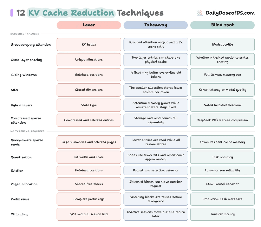
Start with the constraint you need to change, then pick the technique that handles it.
To dive deeper into the full LLMOps lifecycle, we have covered every bit of it in the LLMOps course, starting from fundamentals to production:
Read Part 2 on understanding the core building blocks of LLMs →
Read Part 11 on evaluation of multi-turn systems, tool use evaluations, tracing, and red teaming →
👉 Over to you: how do you reduce KV cache in production?
Good day!