L2 Regularization is Much More Magical That Most People Think

An untaught advantage of L2 regularization that most data scientists don't know.

Almost every tutorial/course/blog mentioning L2 regularization I have seen talks about just one thing:

L2 regularization is a machine learning technique that avoids overfitting by introducing a penalty term into the model’s loss function based on the squares of the model’s parameters.

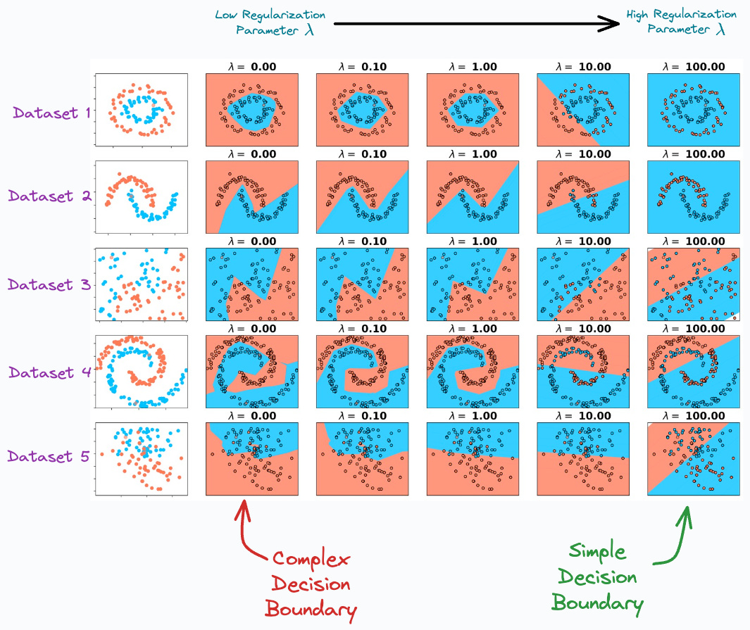
In classification tasks, for instance, increasing the effect of regularization will produce simpler decision boundaries.

---

Of course, the above statements are indeed correct, and I am not denying that.

In fact, we can also verify this from the diagram below:

In the image above, as we move to the right, the regularization parameter increases, and the model creates a simpler decision boundary on all 5 datasets.

---

Coming back to the topic…

However, what disappoints me the most is that most resources don’t point out that L2 regularization is a great remedy for multicollinearity.

Multicollinearity arises when two (or more) features are highly correlated OR two (or more) features can predict another feature:

When we use L2 regularization in linear regression, the algorithm is also called Ridge regression.

But how does L2 regularization eliminate multicollinearity?

Today, let me provide you a demonstrative intuition into this topic, which will also explain why “ridge regression” is called “ridge regression.”

Let’s begin!

---

Dummy dataset

For demonstration purposes, consider this dummy dataset of two features:

As shown above, we have intentionally made featureB highly correlated with featureA. This gives us a dummy dataset to work with.

Going ahead, we shall be ignoring any intercept term for simplicity.

---

Linear regression without L2 penalty

During regression modeling, the goal is to determine those specific parameters (θ₁, θ₂), which minimizes the residual sum of squares (RSS):

So how about we do the following:

• We shall plot the RSS value for many different combinations of (θ₁, θ₂) parameters. This will create a 3D plot:

  • x-axis → θ₁

  • y-axis → θ₂

  • z-axis → RSS value

• Next, we shall visually assess this plot to locate those specific parameters (θ₁, θ₂) that minimize the RSS value.

Let’s do this.

Without the L2 penalty, we get the following plot (it’s the same plot but viewed from different angles):

Did you notice something?

The 3D plot has a valley. There are multiple combinations of parameter values (θ₁, θ₂) for which RSS is minimum.

Thus, obtaining a single value for the parameters (θ₁, θ₂) that minimize the RSS is impossible.

---

Linear regression with L2 penalty

When using an L2 penalty, the goal is to minimize the following:

Creating the same plot again as we did above, we get the following:

Did you notice something different this time?

As depicted above, using L2 regularization removes the valley we saw earlier and provides a global minima to the RSS error.

Now, obtaining a single value for the parameters (θ₁, θ₂) that minimizes the RSS is possible.

Out of nowhere, L2 regularization helped us eliminate multicollinearity.

---

Why the name “ridge regression”?

In fact, this is where “ridge regression” also gets its name from — it eliminates the ridge in the likelihood function when the L2 penalty is used.

Of course, in the demonstrations we discussed earlier, we noticed a valley, not a ridge.

However, in that case, we were considering the residual sum of error — something which is minimized to obtain the optimal parameters.

Thus, the error function will obviously result in a valley.

If we were to use likelihood instead — something which is maximized, it would (somewhat) invert the graph upside down and result in a ridge instead:

Apparently, while naming the algorithm, the likelihood function was considered.

And that is why it was named “ridge regression.”

Pretty cool, right?

When I first learned about this some years back, I literally had no idea that such deep thought went into naming ridge regression.

Hope you learned something new today :)

If you want to learn about the probabilistic origin of L2 regularization, check out this article: The Probabilistic Origin of Regularization.

👉 Over to you: What are some other advantages of using L2 regularization?

---

👉 If you liked this post, don’t forget to leave a like ❤️. It helps more people discover this newsletter on Substack and tells me that you appreciate reading these daily insights.

Thanks so much for appreciating the effort :)

The button is located towards the bottom of this email.

Thanks for reading!

---

Latest full articles

If you’re not a full subscriber, here’s what you missed recently:

• Don’t Stop at Pandas and Sklearn! Get Started with Spark DataFrames and Big Data ML using PySpark.

• DBSCAN++: The Faster and Scalable Alternative to DBSCAN Clustering

• Federated Learning: A Critical Step Towards Privacy-Preserving Machine Learning

• You Cannot Build Large Data Projects Until You Learn Data Version Control!

• Sklearn Models are Not Deployment Friendly! Supercharge Them With Tensor Computations.

Use this decision tree to decide:

To receive all full articles and support the Daily Dose of Data Science, consider subscribing below:

---

👉 Tell the world what makes this newsletter special for you by leaving a review here :)

👉 If you love reading this newsletter, feel free to share it with friends!