MLE vs. EM — What’s the Difference?
A popular interview question.
Maximum likelihood estimation (MLE) and expectation maximization (EM) are two popular techniques to determine the parameters of statistical models.
Due to its applicability in MANY statistical models, I have seen it being asked in plenty of data science interviews as well, especially the distinction between the two.
So today, let’s understand them in detail, how they work, and their differences.
Let’s begin!
Maximum likelihood estimation (MLE)
MLE starts with a labeled dataset and aims to determine the parameters of the statistical model we are trying to fit.
The process is pretty simple and straightforward.
In MLE, we:
Start by assuming a data generation process. Simply put, this data generation process reflects our belief about the distribution of the output label (
y), given the input (X).
Next, we define the likelihood of observing the data. As each observation is independent, the likelihood of observing the entire data is the same as the product of observing individual observations:
The likelihood function above depends on parameter values (θ). Our objective is to determine those specific parameter values that maximize the likelihood function. We do this as follows:
This gives our parameter estimates that would have most likely generated the given data.
That was pretty simple, wasn’t it?
But what do we do if we don’t have true labels?
We still want to estimate the parameters, don’t we?
MLE, as you may have guessed, will not be applicable. The true label (y), being unobserved, makes it impossible to define a likelihood function like we did earlier.
In such cases, advanced techniques like expectation maximization are pretty helpful.
Expectation maximization (EM)
EM is an iterative optimization technique to estimate the parameters of statistical models. It is particularly useful when we have an unobserved (or hidden) label.
One example situation could be as follows:
As depicted above, we assume that the data was generated from multiple distributions (a mixture). However, the observed/complete data does not contain that information.
In other words, the observed dataset does not have information about whether a specific row was generated from distribution 1 or distribution 2.
Had it contained the label (
y) information, we would have already used MLE.
EM helps us with parameter estimates of such datasets.
The core idea behind EM is as follows:
Make a guess about the initial parameters (θ).
Expectation (E) step: Compute the posterior probabilities of the unobserved label (let’s call it ‘
z’) using the above parameters.Here, ‘
z’ is also called a latent variable, which means hidden or unobserved.Relating it to our case, we know that the true label exists in nature. But we don’t know what it is.
Thus, we replace it with a latent variable ‘
z’ and estimate its posterior probabilities using the guessed parameters.
Given that we now have a proxy (not precise, though) for the true label, we can define an “expected likelihood” function. Thus, we use the above posterior probabilities to do so:
Maximization (M) step: So now we have a likelihood function to work with. Maximizing it with respect to the parameters will give us a new estimate for the parameters (θ`).
Next, we use the updated parameters (θ`) to recompute the posterior probabilities we defined in the expectation step.
We will update the likelihood function (
L) using the new posterior probabilities.Again, maximizing it will give us a new estimate for the parameters (θ).
And this process goes on and on until convergence.
The point is that in expectation maximization, we repeatedly iterate between the E and the M steps until the parameters converge.
A good thing about EM is that it always converges. Yet, at times, it might converge to a local extrema.
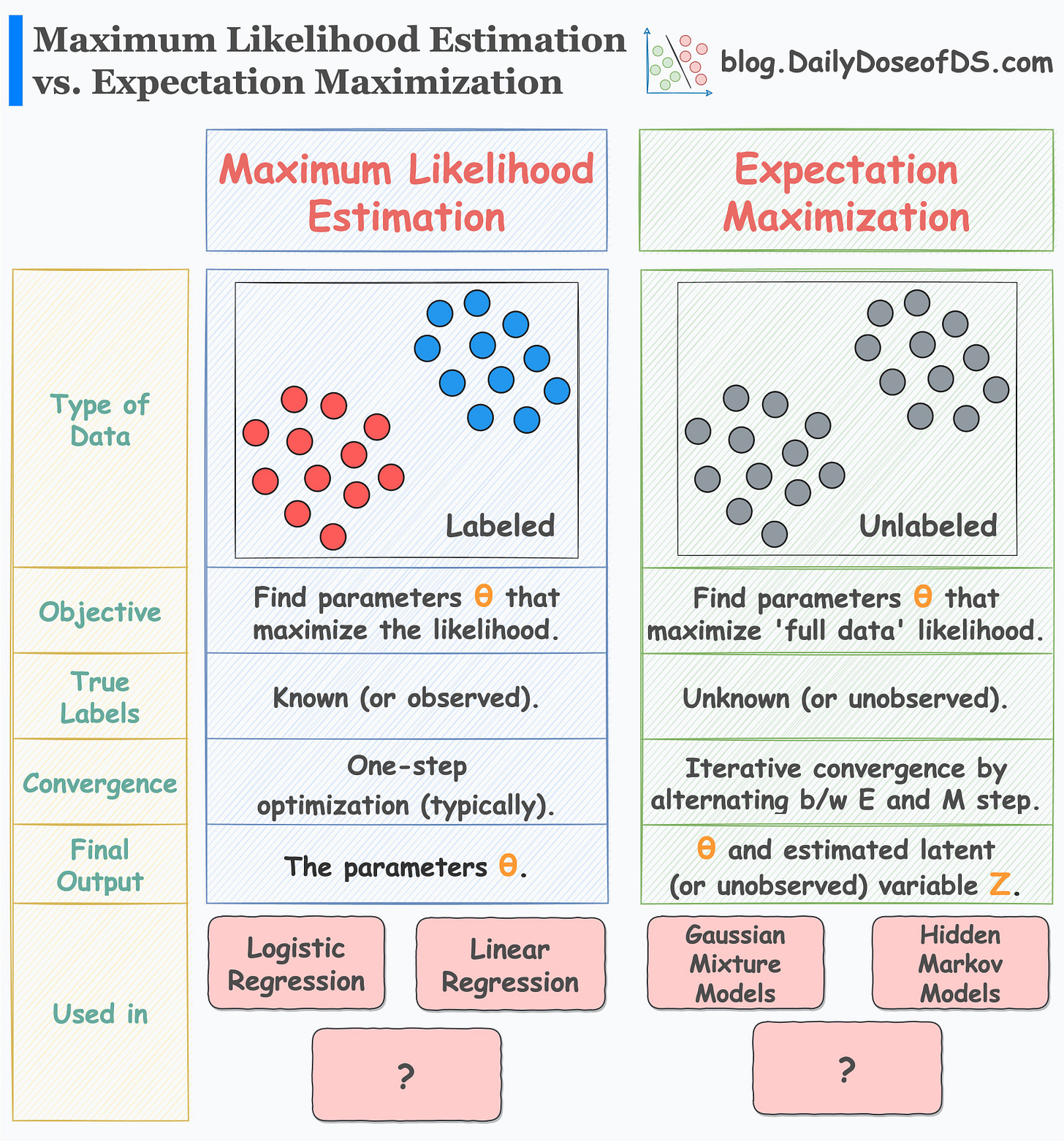
I prepared the following visual, which neatly summarizes the differences between MLE and EM:
MLE vs. EM is a popular question asked in many data science interviews.
While MLE is relatively easy to understand, EM is a bit complicated.
If you are interested in practically learning about expectation maximization and programming it from scratch in Python (using only NumPy)...
….then we covered it in detail in this deep dive: Gaussian Mixture Models: The Flexible Twin of KMeans.
👉 Over to you: In the above visual summary, can you add more models for each MLE and EM?
👉 If you liked this post, don’t forget to leave a like ❤️. It helps more people discover this newsletter on Substack and tells me that you appreciate reading these daily insights.
The button is located towards the bottom of this email.
Thanks for reading!
Latest full articles
If you’re not a full subscriber, here’s what you missed last month:
PyTorch Models Are Not Deployment-Friendly! Supercharge Them With TorchScript.
How To (Immensely) Optimize Your Machine Learning Development and Operations with MLflow.
Don’t Stop at Pandas and Sklearn! Get Started with Spark DataFrames and Big Data ML using PySpark.
DBSCAN++: The Faster and Scalable Alternative to DBSCAN Clustering.
Federated Learning: A Critical Step Towards Privacy-Preserving Machine Learning.
You Cannot Build Large Data Projects Until You Learn Data Version Control!
Deploy, Version Control, and Manage ML Models Right From Your Jupyter Notebook with Modelbit.
To receive all full articles and support the Daily Dose of Data Science, consider subscribing:
👉 Tell the world what makes this newsletter special for you by leaving a review here :)
👉 If you love reading this newsletter, feel free to share it with friends!


Excellent article for the difference between two techniques
Absolutely brilliant! Thanks for writing a great article!!