Never Use PCA for Visualization Unless This Specific Condition is Met
Using variance as an indicator for visualization.
PCA, by its very nature, is a dimensionality reduction technique.
The core idea is to project the data to some other space using the eigenvectors of the covariance matrix.
This creates uncorrelated features, each of which explains some amount of original data variance.
Yet, at times, many use PCA for visualizing high-dimensional datasets.
This is done by projecting the given data into two dimensions and visualizing it.
While this may appear like a fair thing to do, there’s a big problem here that often gets overlooked.
After applying PCA, each new feature captures a fraction of the original variance.
This means that two-dimensional visualization will only be useful if the first two principal components collectively capture most of the original data variance.
If not, the two-dimensional visualization will be highly misleading and incorrect. This is because the first two components don’t capture the majority of the original variance well.
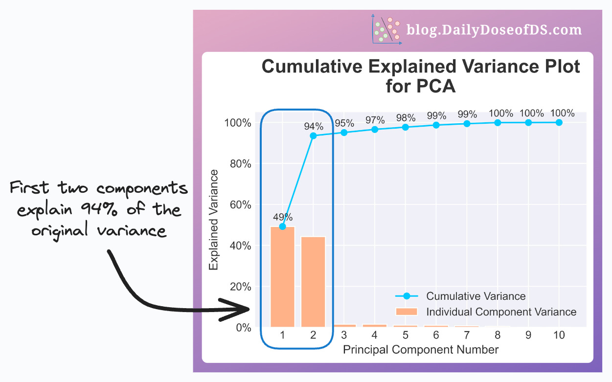
You can prevent this mistake by first plotting a cumulative explained variance plot.
As the name suggests, it plots the cumulative variance explained by principal components.
In the plot below, the first two components only explain 56% of the original data variance.
Thus, visualizing this dataset in 2D using PCA may not be a good choice because plenty of data variance is missing.
However, in the below plot, the first two components explain 94% of the original data variance.
Thus, using PCA for visualization will be a good choice.
As a takeaway, use PCA for 2D visualization only when the above plot suggests so. If not, refrain from using PCA for 2D visualization.
That being said, it is true that PCA is the most commonly used technique for dimensionality reduction.
Despite its popularity, most folks struggle to design its true end-to-end formulation from scratch.
Many try to explain PCA by relating it to the idea of eigenvectors and eigenvalues, which is true — PCA does perform transformations using eigenvectors and eigenvalues.
But why?
In other words, where did this whole notion of eigenvectors and eigenvalues originate from in PCA?
There are a few questions to ask here:
Why do eigenvectors even show up in PCA?
How can we be sure that the data projections using eigenvectors is the most obvious solution to proceed with?
How can we be sure that the above transformation does preserve the entire data variance?
How can we be sure that the new features are indeed uncorrelated?
Can you answer these questions?
If not, then this is precisely the topic of today’s machine learning deep dive: Formulating the Principal Component Analysis (PCA) Algorithm From Scratch.
Very few know that the above solution of PCA naturally appears from an optimization step, which PCA tries to maximize during its projections.
Yes, the formulation of PCA involves an optimization step too — derivatives and everything...
Yet, most resources never elaborate on this.
Thus, today’s article covers:
The intuition and the motivation behind dimensionality reduction.
What are vector projections and how do they alter the mean and variance of the data?
What is the optimization step of PCA?
What are Lagrange Multipliers?
How are Lagrange Multipliers used in PCA optimization?
What is the final solution obtained by PCA?
Proving that the new features are indeed uncorrelated.
How to determine the number of components in PCA?
What are the advantages and disadvantages of PCA?
Key takeaway.
👉 Interested folks can read it here: Formulating the Principal Component Analysis (PCA) Algorithm From Scratch.
Hope you will learn something new today :)
👉 If you liked this post, don’t forget to leave a like ❤️. It helps more people discover this newsletter on Substack and tells me that you appreciate reading these daily insights. The button is located towards the bottom of this email.
Thanks for reading :)


