

In today’s newsletter:
Training LLMs without one correct answer.
Prefix-aware LLM routing, clearly explained.
Regular ML Inference vs. LLM Inference
Training LLMs without one correct answer
Suppose a model must translate questions from finance analysts into SQL.
A basic verifier might run each generated query and return a reward of 1 when it executes without an error.
Due to this, the model will learn to produce executable SQL, but it will not necessarily learn to produce correct SQL.
A query can select the wrong columns, omit a filter, duplicate rows after a join, or calculate revenue over the wrong period. The database will execute all of them without complaint.
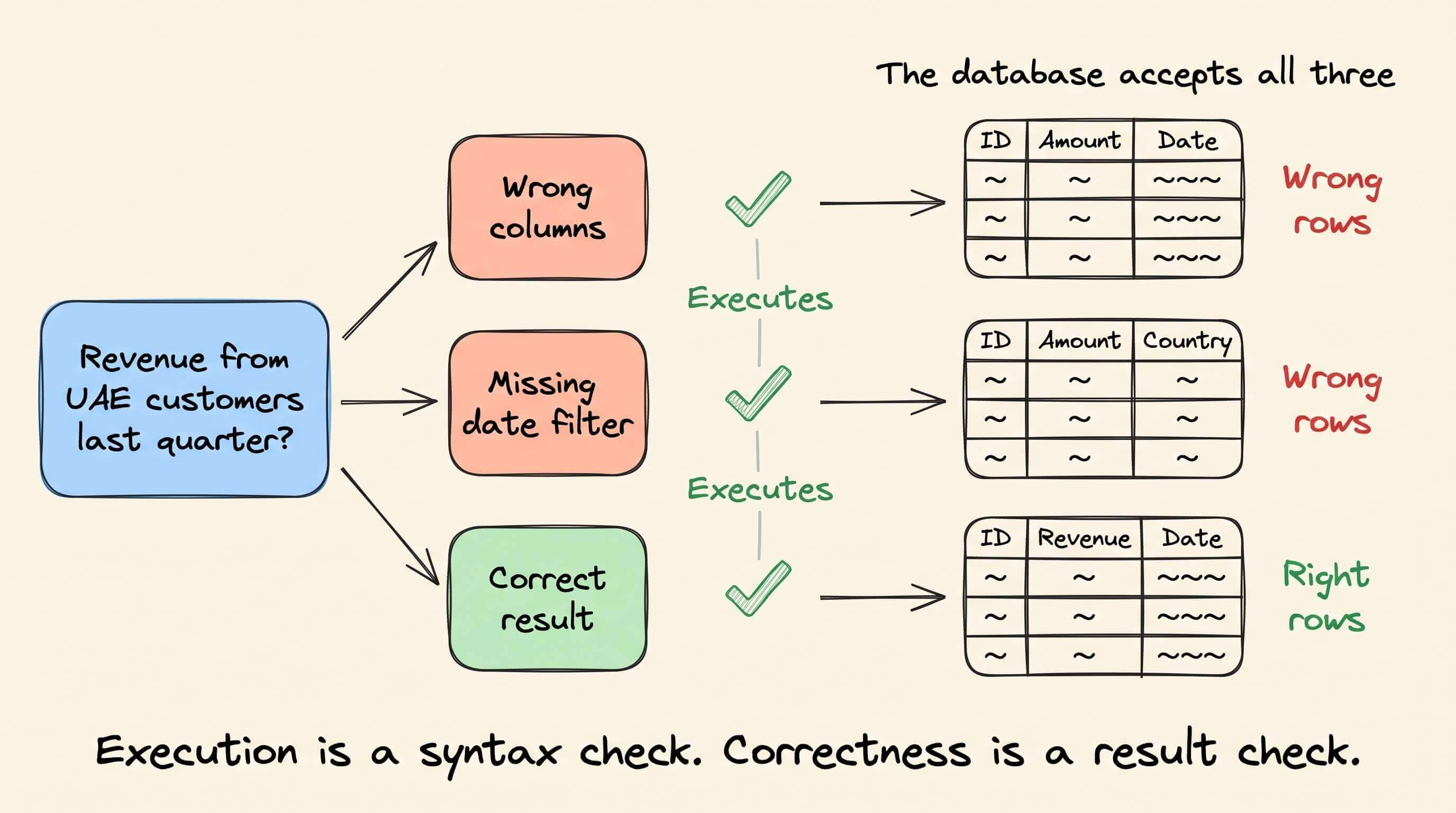
This is the part of RLVR that deserves more attention. A verifier inherently does not discover what correctness means, which is why the engineer must encode it.
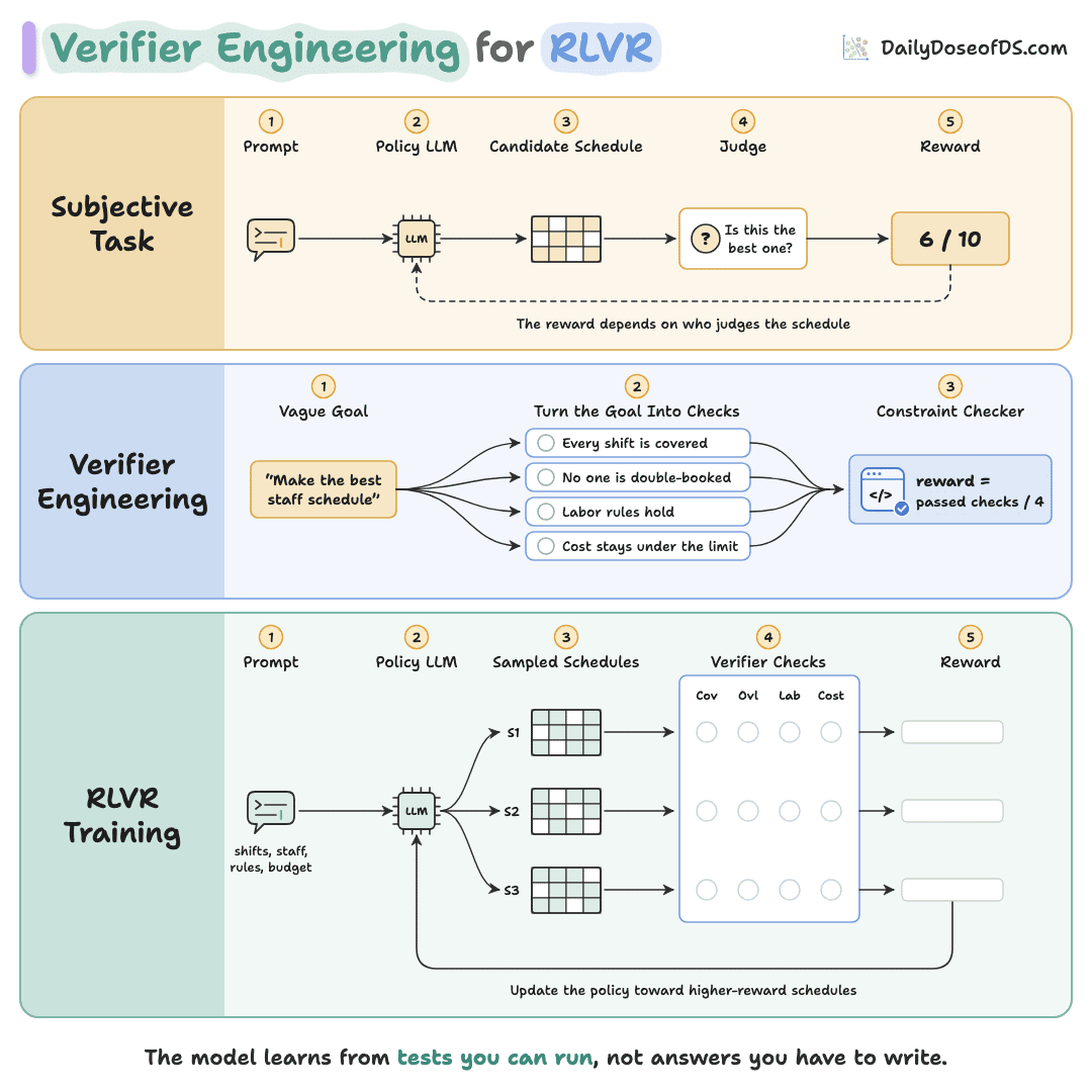
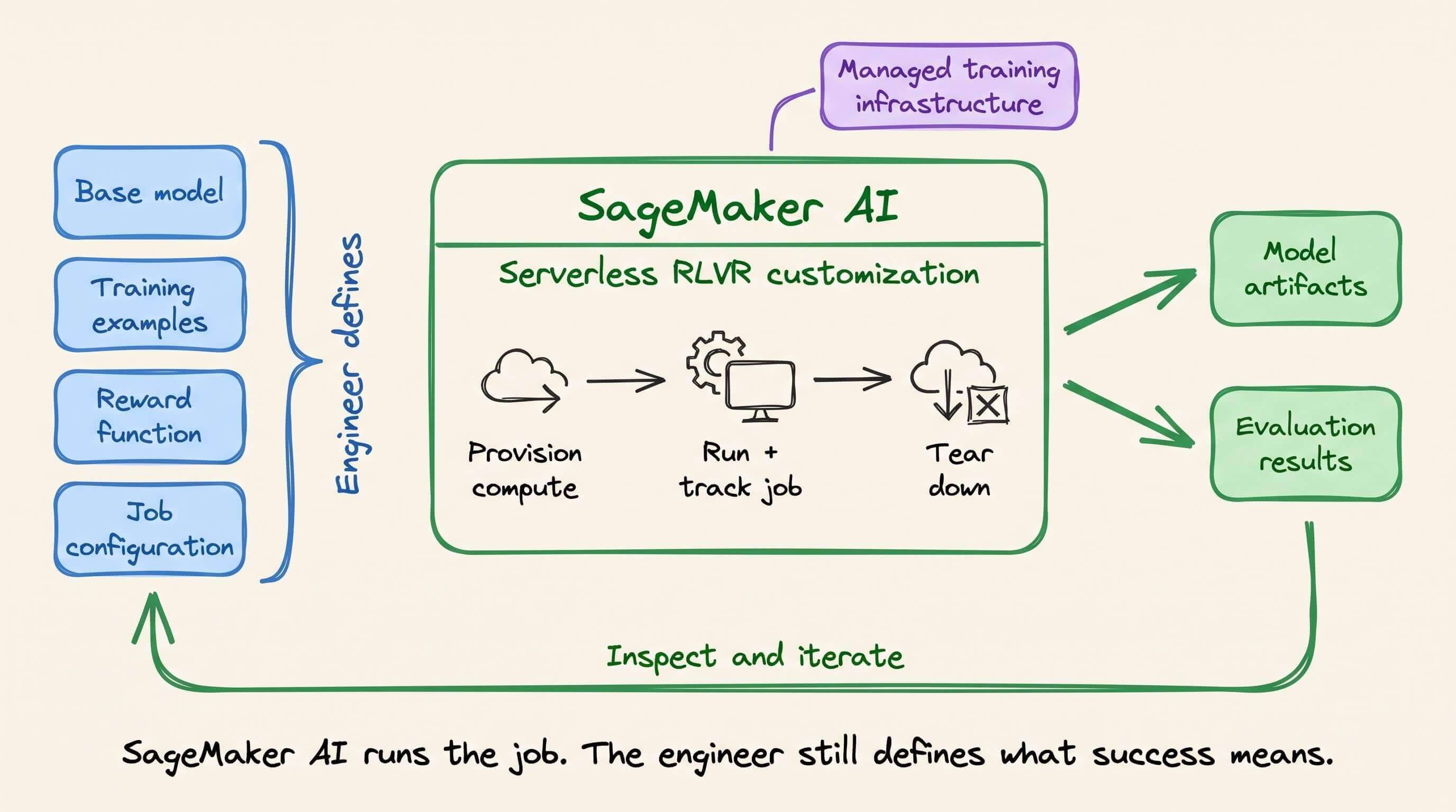
Amazon SageMaker AI makes it simple to test that definition through its serverless model customization workflow.
In SageMaker Studio, the engineer can select a base model, prepare the examples, attach a custom reward function, and submit an RLVR job without managing the training infrastructure.
SageMaker AI provisions the compute, runs and tracks the job, stores the resulting model artifacts, and tears the infrastructure down afterward.
That makes it easier to iterate on the model and reward logic as separate parts of the experiment.
For text-to-SQL, you can split the verifier into layers.
The first layer checks whether the query parses, executes, and remains read-only.
The second compares the returned rows with the reference result. This catches queries that are valid SQL but answer a different question.
The final layer can score operational properties such as latency or scanned data, but only after the query has passed the correctness checks.
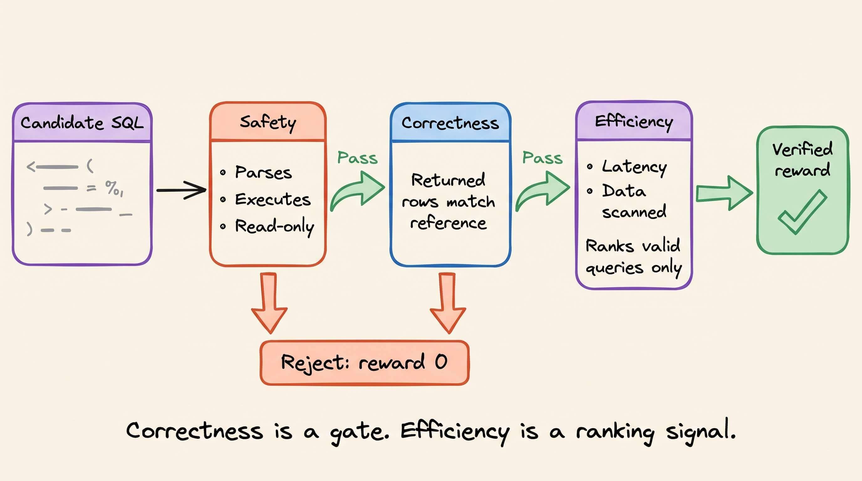
The order is important because a fast query that returns the wrong rows should never outrank a slower query that returns the right ones.
During customization, the model generates several candidates for each prompt. The verifier scores them, and GRPO updates the model toward the candidates that satisfy the full specification.
This also gives the evaluation stage a clear purpose. A higher training reward is not enough. The customized model must improve on held-out execution accuracy without increasing unsafe queries or weakening result correctness.
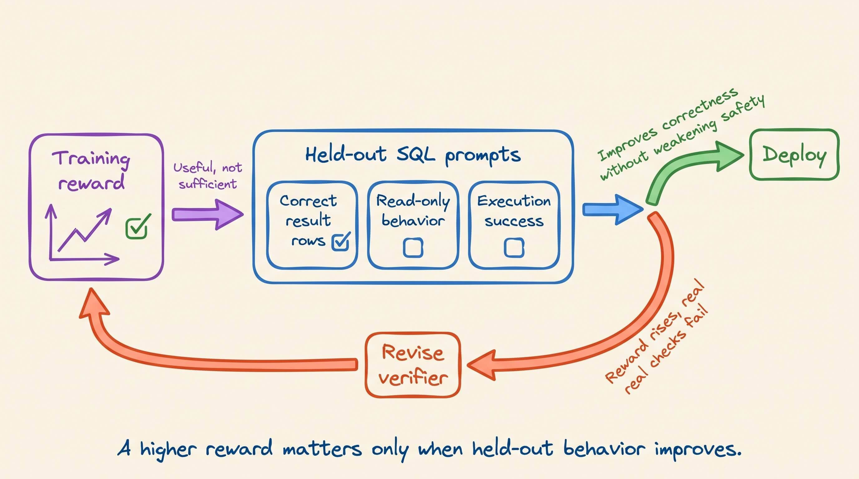
SageMaker AI agent skills can help with model selection, data preparation, job configuration, evaluation, and deployment through Claude Code, Codex, Kiro, or another compatible coding agent.
AWS has published an interactive workshop for anyone who wants to get hands-on with serverless model customization in SageMaker AI:
Try the SageMaker AI model customization workshop →
Thanks to AWS for working with us on today’s issue!
Prefix-Aware LLM Routing, clearly explained
The same request on the same GPUs can wait 92 seconds or half a second for its first token, depending only on where the router sends it.
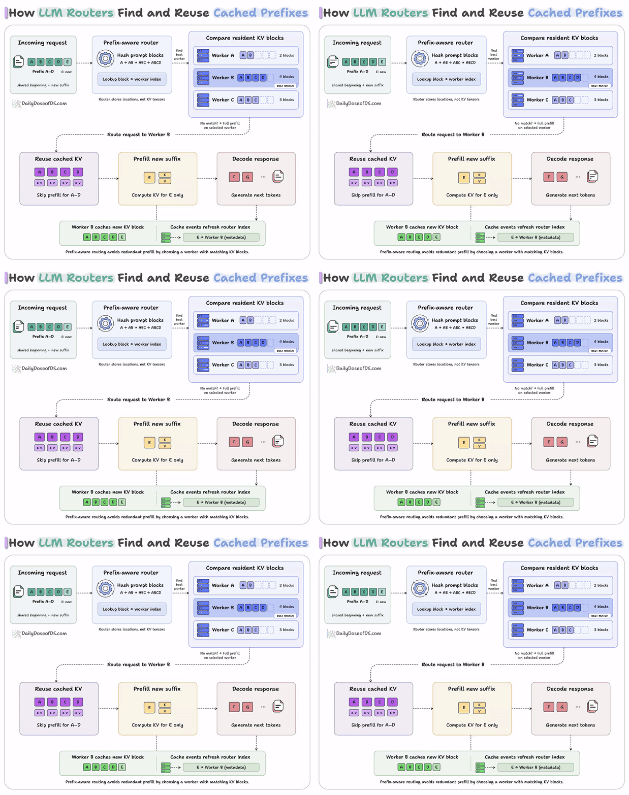
Production prompts start with the same system prompt, tool definitions and earlier turns. Only the last part of each request is new.
So the GPU that served the previous turn still holds the KV cache for that shared prefix.
But a cache-blind router may send the next request to a different GPU, which then recomputes the whole prefix before it can write a single token.
A prefix-aware router avoids this by tracking which GPU holds which part of each prompt.
Let’s walk through how it works.
1. Why routing decides the cache hit
Inside one engine, prefix caching already works well. In llm-d’s tests, sending a roughly 10,000-token prompt to a Qwen3-32B vLLM instance a second time cut time to first token from 4.3s to 0.6s.
The trouble starts when we scale out. Each replica keeps its own KV cache, and no replica can see another’s.
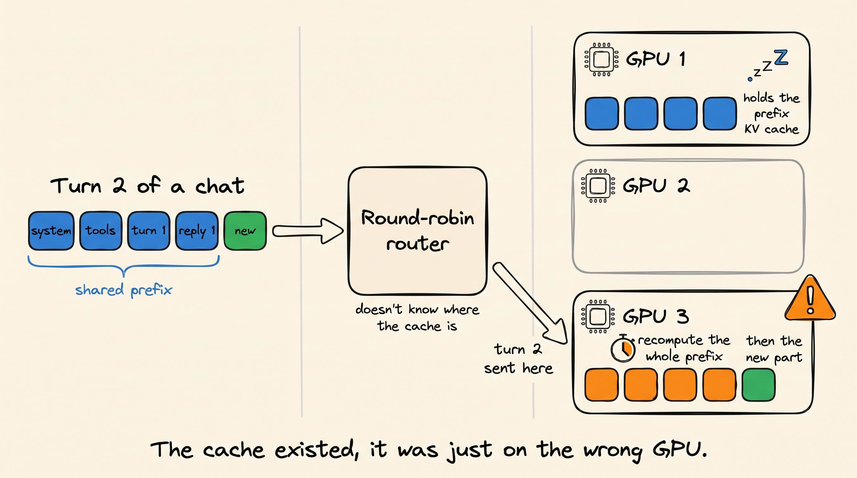
With 8 replicas and random routing, the next turn lands on the warm GPU about 1 time in 8.
The other 7 times, a GPU recomputes a prefix that already sits in memory somewhere else in the cluster.
So in a cluster, the router decides whether the engine’s prefix cache gets used at all.
2. Hash the prompt block by block
The engine stores the KV cache in fixed-size blocks. vLLM uses 16 tokens per block by default and only caches full blocks.
Each block gets a hash built from its parent block’s hash plus its own token IDs. So the hash of block D covers A, B, C and D together.
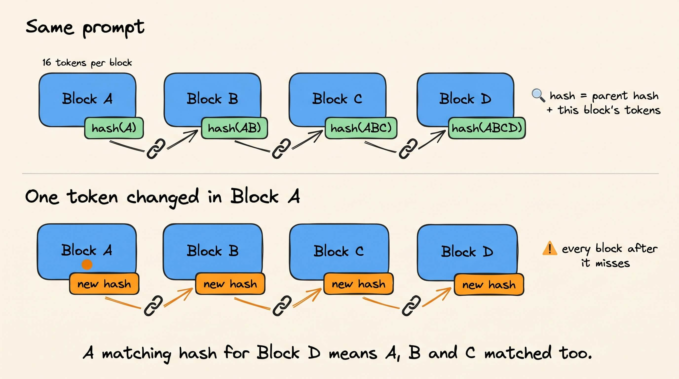
Here is a simplified version of what vLLM does:
def block_hashes(token_ids, block_size=16):
    hashes, parent = [], None
    for i in range(0, len(token_ids) - block_size + 1, block_size):
        block = tuple(token_ids[i:i + block_size])
        parent = hash((parent, block))
        hashes.append(parent)
    return hashes
This chaining turns a block lookup into a prefix lookup. If block D’s hash matches, everything before it matched too.
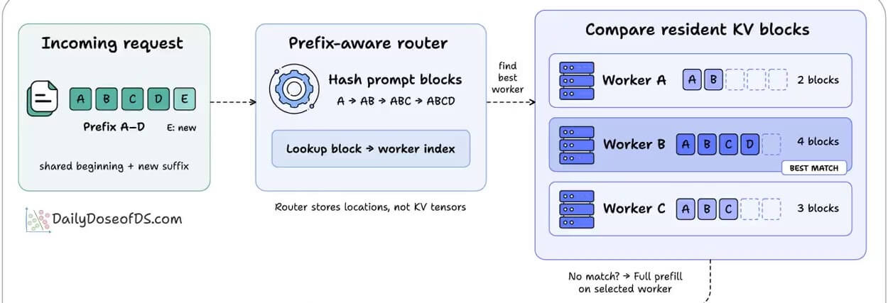
The router computes the same hashes for each incoming request, so it can compare prompts without touching any KV tensors.
3. Look up which worker holds those blocks
The router keeps a block-to-worker index. It maps each block hash to the workers that hold that block, and it never stores the KV tensors themselves.
That keeps the index tiny. llm-d ran the numbers for DeepSeek-R1 in FP8 on 8 H200s, where each 128-token block takes about 8.6 MB of VRAM but only an 8-byte hash in the index.
So a 365 GB KV cache pool needs only about 339 KB of index.
For a request with prefix blocks A to D and a new suffix E, the router walks the hashes in order:
↳ Worker A holds 2 matching blocks.
↳ Worker C holds 3.
↳ Worker B holds all 4, so Worker B gets the request.
If no worker has a match, the request gets a full prefill on whichever worker the router picks.
4. Reuse the cache and report back
Worker B reuses the cached KV for A to D, computes KV only for E, and starts decoding.
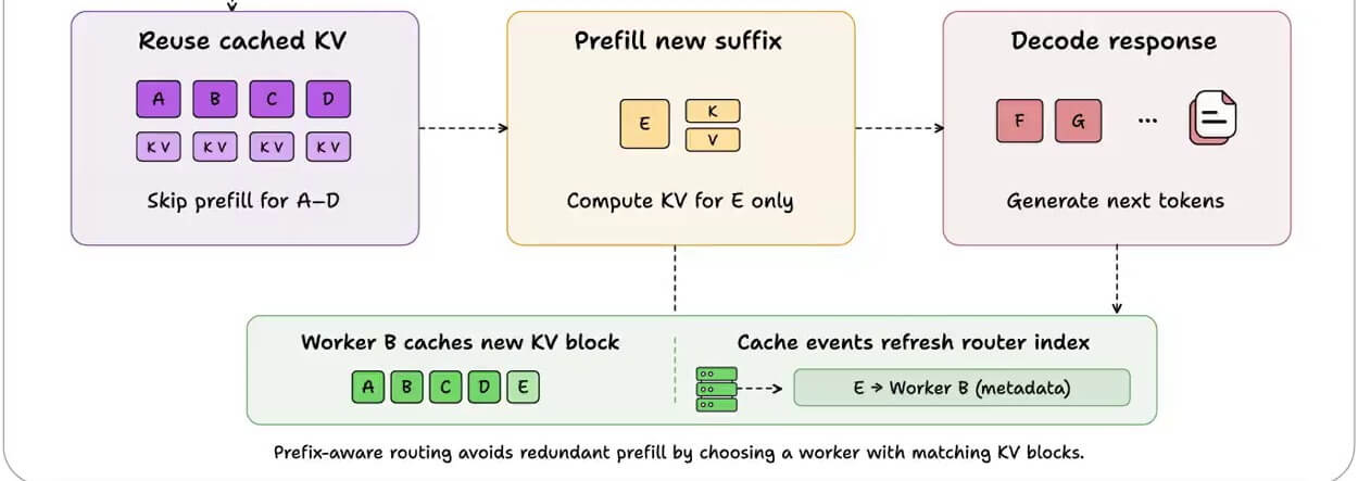
Once E is cached, Worker B emits a cache event and the router records that E now lives on Worker B. So the next turn of this conversation lands on Worker B too.
Evictions emit events as well. In llm-d, each vLLM pod publishes these KV events over ZMQ every time a block is created or evicted, so the index tracks what each GPU actually holds.
That is the difference between precise and approximate routing. An approximate router guesses cache locations from its own routing history instead.
5. Weigh load against cache hits
If the router only chased cache matches, the warmest GPU would end up with the longest queue, because every matching request wants it.
So real routers score load too. NVIDIA Dynamo’s KV router adds the prefill a worker would still owe after cache credit to that worker’s decode load, then picks the lowest total.
Here is the example from Dynamo’s docs, for a request with 10 prefill blocks:
cost = (prefill blocks - cached blocks) + decode blocks

Worker 1: (10 - 2) + 10 = 18
Worker 2: (10 - 5) + 5  = 10   <- picked
Worker 3: (10 - 8) + 9  = 11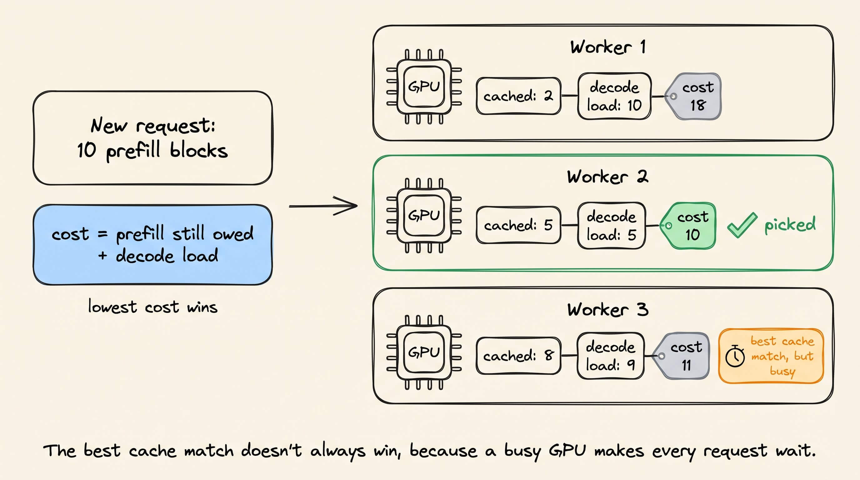
Worker 3 has the best match, yet Worker 2 wins. The router accepts recomputing 3 extra blocks to avoid the busier GPU.
Dynamo exposes this tradeoff as a knob. More cache credit lowers time to first token, and less credit spreads load more evenly and lowers inter-token latency.
llm-d compared four routing strategies on 8 vLLM pods across 16 H100s.
The workload simulated 150 customers, each with a 6,000-token shared context and 5 users sending 1,200-token questions, at 3 to 60 QPS. Those shared prefixes needed about 73% of the cluster’s KV cache, roughly 6x what one pod could hold.
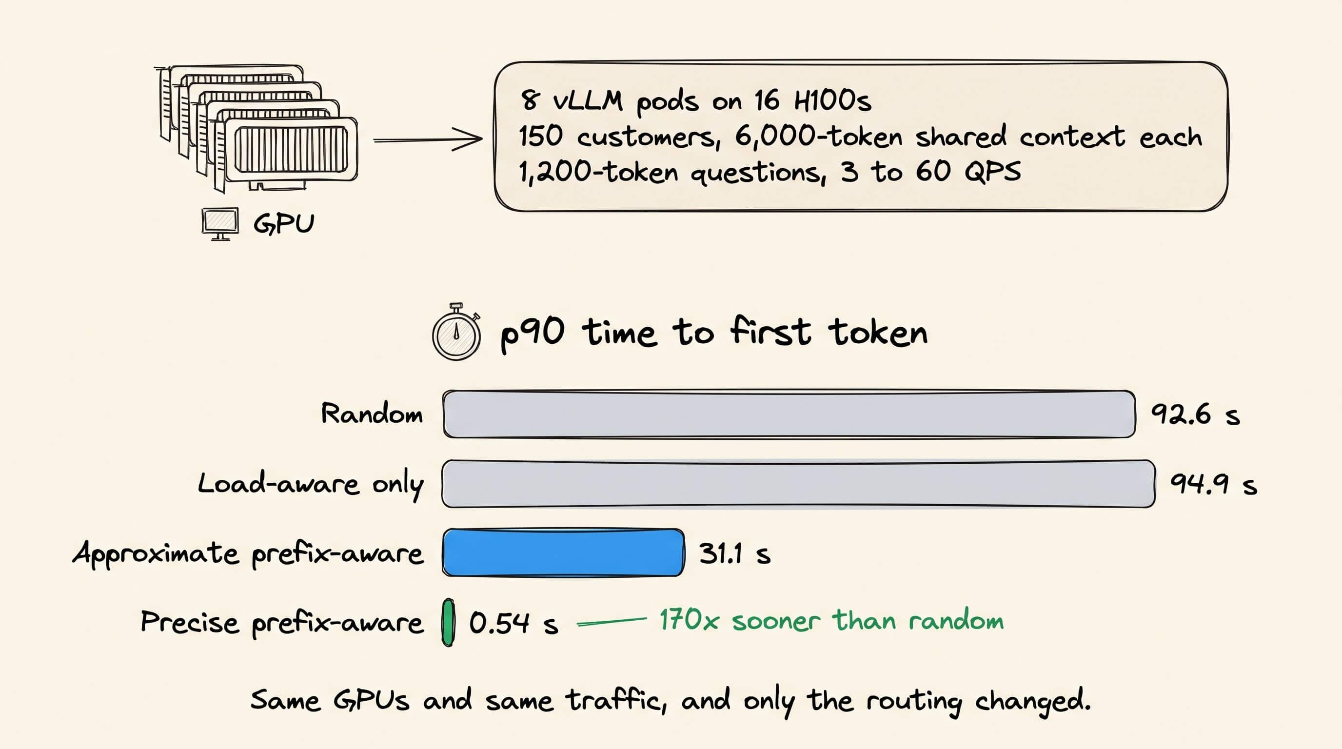
Here are the p90 times to first token:
Random: 92.6s
Load-aware only: 94.9s
Approximate prefix-aware: 31.1s
Precise prefix-aware: 0.54s
That is about 170x sooner than random routing. Output throughput also roughly doubled, from 4,429 to 8,730 tokens/s.
Load-aware routing did no better than random. Spreading requests evenly doesn’t help when each one lands on a GPU that has to recompute its prefix.
A later llm-d rerun on a newer vLLM, against a plain Kubernetes round-robin Service, showed a smaller gap, but p90 time to first token still dropped by more than 99%.
All of this depends on the prefix cache itself working.
A small change early in the prompt, like a timestamp at the top of the system prompt, changes every block hash after it, and no router can match those blocks.
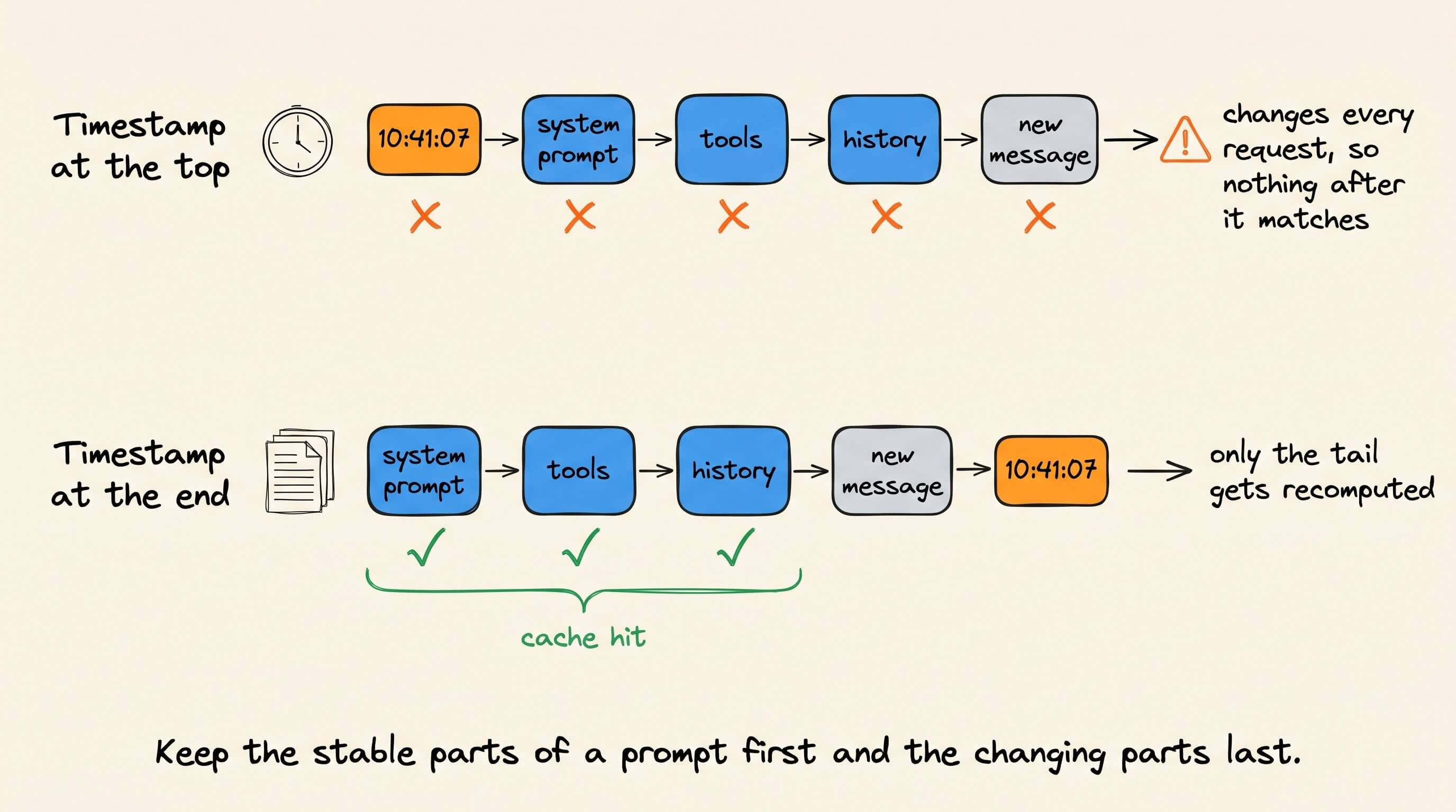
So keep the stable parts first, like the system prompt, tool definitions, and documents. Put whatever changes per request at the end.
A router can only find a cached prefix if the prompt still produces the same hashes.
We covered how prefix caching works, how it differs from KV, prompt, and semantic caching, and which prompt changes cause cache misses, in a detailed article.
👉 Over to you: Does your serving stack route requests by cache location, or does it still round-robin across replicas?
Regular ML inference vs. LLM inference
LLM inference presents unique challenges over regular ML inference, due to which we have specialized, high-performance LLM inference engines, like vLLM, LMCache, SGLang, and TensorRT-LLM.
Let’s understand these challenges today and how we solve them!
Continuous batching
Traditional models, like CNNs, usually deal with a fixed-size image input and a fixed-length output (like a label). This makes batching easy.

LLMs, however, deal with variable-length inputs (the prompt) and generate variable-length outputs.

So if you batch some requests, all will finish at different times, and the GPU would have to wait for the longest request to finish before it can process new requests. This leads to idle time on the GPU:
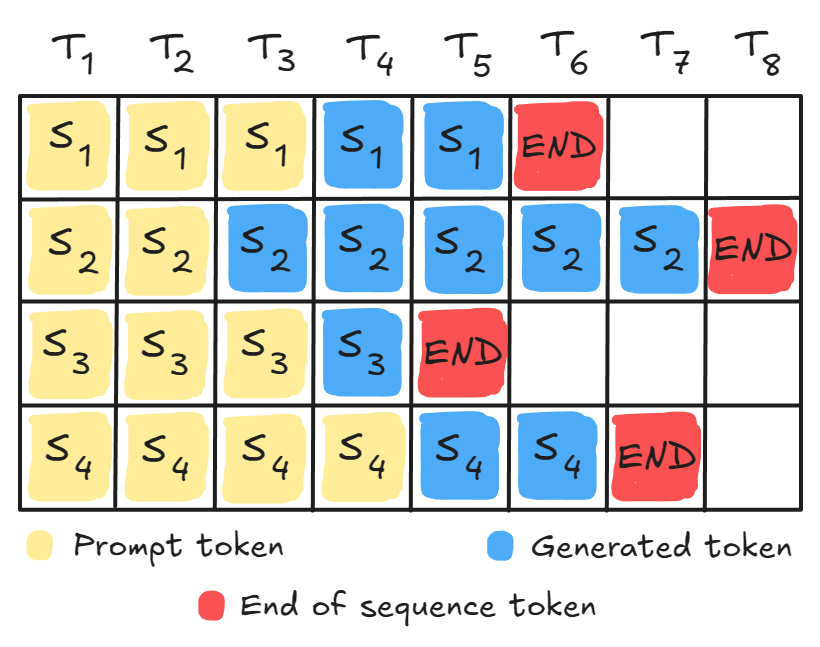
Continuous Batching solves this.

Instead of waiting for the entire batch to finish, the system monitors all sequences and swaps completed ones (<EOS> token) with new queries:
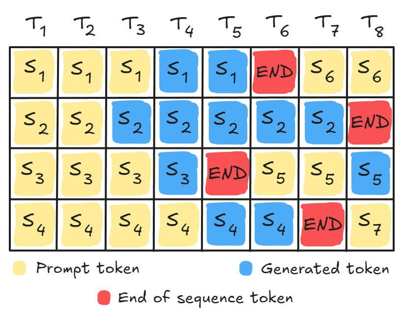
This keeps the GPU pipeline full and maximizes utilization.
Prefill-decode disaggregation
LLM inference is a two-stage process with fundamentally different resource requirements.
The prefill stage processes all the input prompt tokens at once, so this is compute-heavy.
The decode stage autoregressively generates the output, and this demands low latency.

Running both stages on the GPU means the compute-heavy prefill requests will interfere with the latency-sensitive decode requests.
Prefill-decode disaggregation solves this by allocating a dedicated pool of GPUs for the prefill stage and another pool for the decode stage.
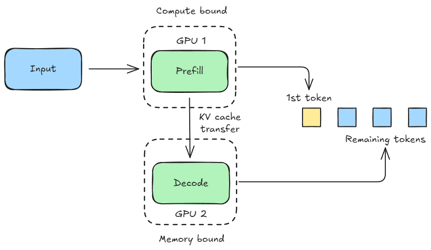
In contrast, a standard ML model typically has a single, unified computation phase.
GPU memory management + KV caching
Generating a new token uses the key and value vectors of all previous tokens. To avoid recomputing these vectors for all tokens over and over, we cache them (we covered KV caching in detail here):
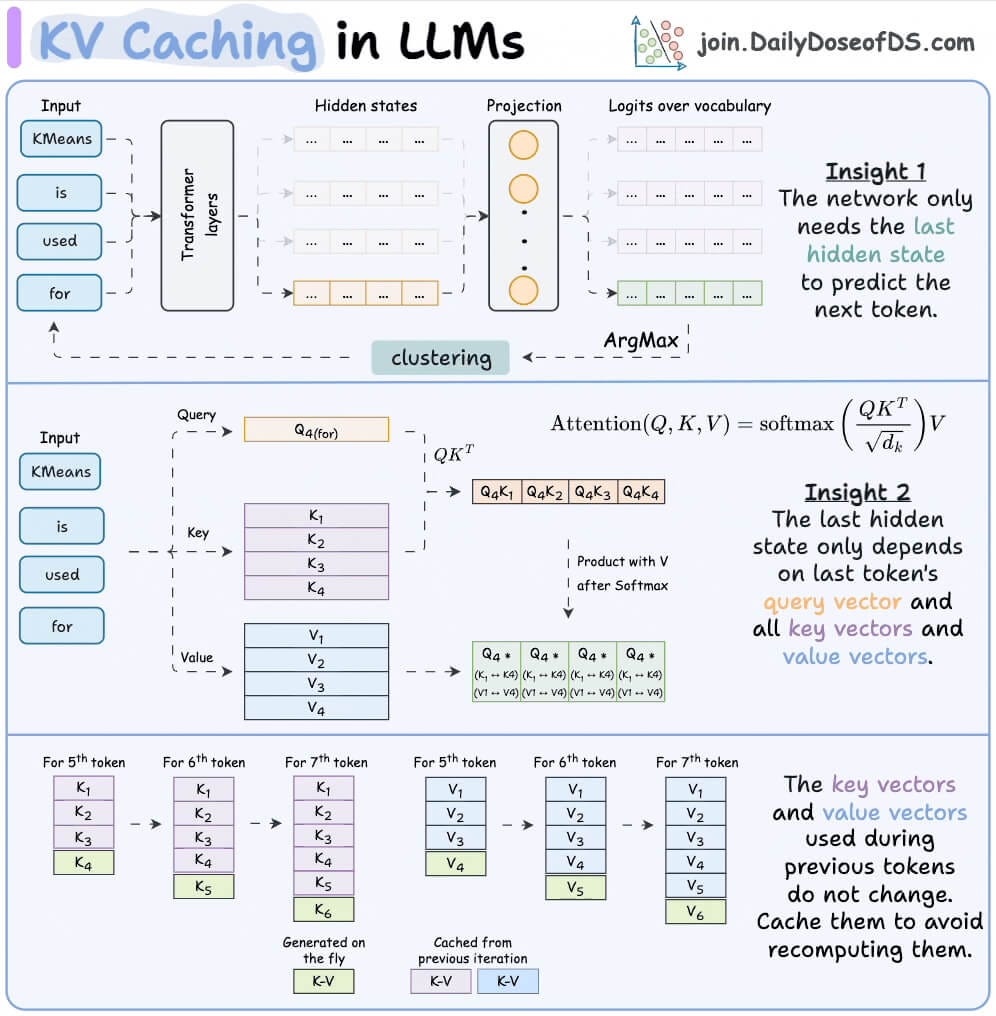
This KV Cache grows linearly with the total length of the conversation history.
But in many workflows, inputs like the system prompts are shared across many requests. So we can avoid recomputing them by using these KV vectors across all chats:
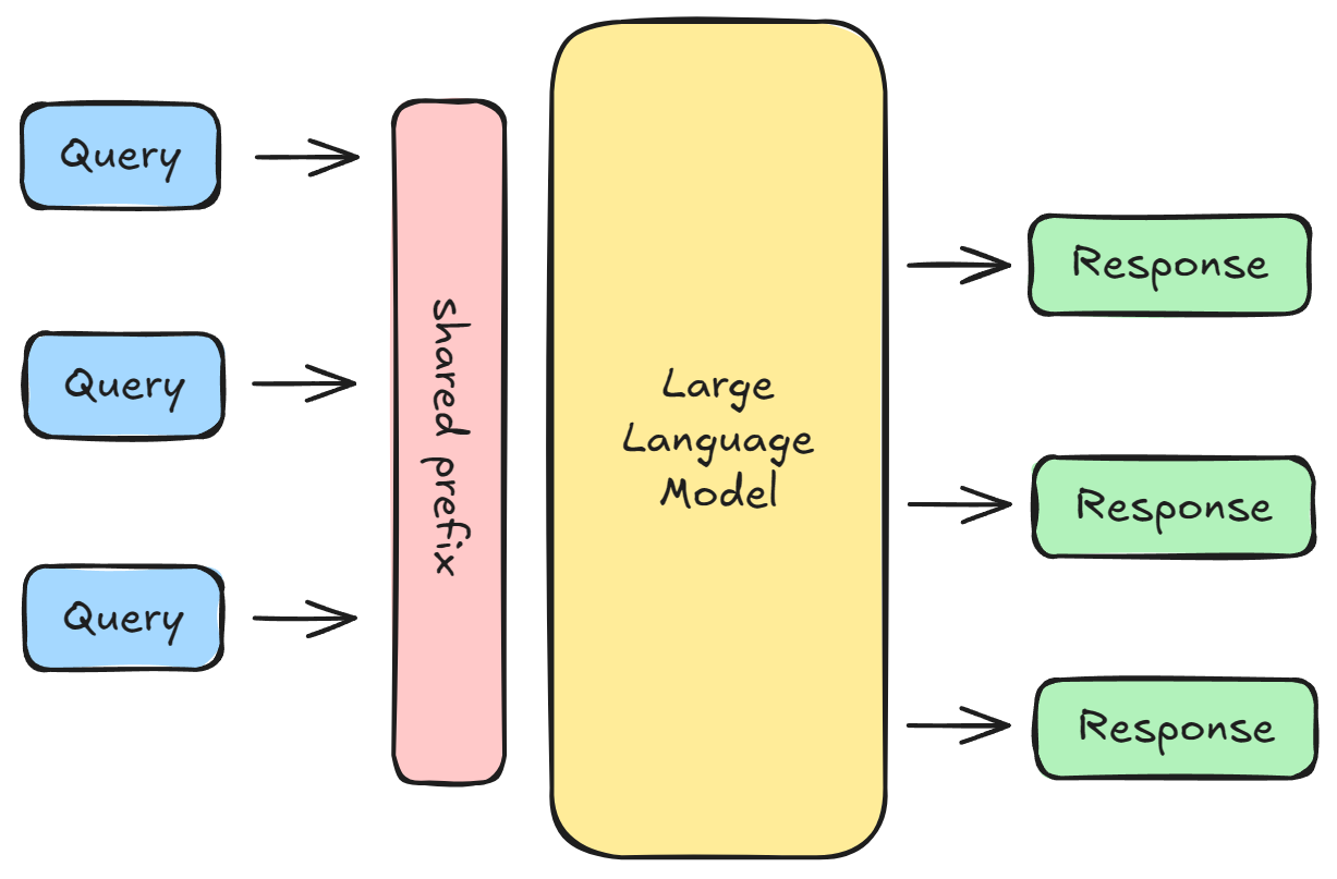
That said, KV cache takes up a significant memory since it’s stored in contiguous blocks. This wastes GPU memory and leads to memory fragmentation:

Paged Attention solves this problem by storing KV caching in non-contiguous blocks and then using a lookup table to track these blocks. The LLM only loads the blocks it needs, instead of loading everything at once.
We will cover Paged Attention in another issue.
Prefix-aware routing
To scale standard ML models, you can simply replicate the model across multiple servers/GPUs and use straightforward load-balancing schemes like Round Robin or routing to the least-busy server.
Since each request is independent, this works fine.
But LLMs heavily rely on caching (like the shared KV prefix discussed above), so requests are no longer independent.
If a new query comes in with a shared prefix that has already been cached on Replica A, but the router sends it to Replica B (which is less busy), Replica B has to recompute the entire prefix’s KV cache.
Prefix-aware routing solves this.
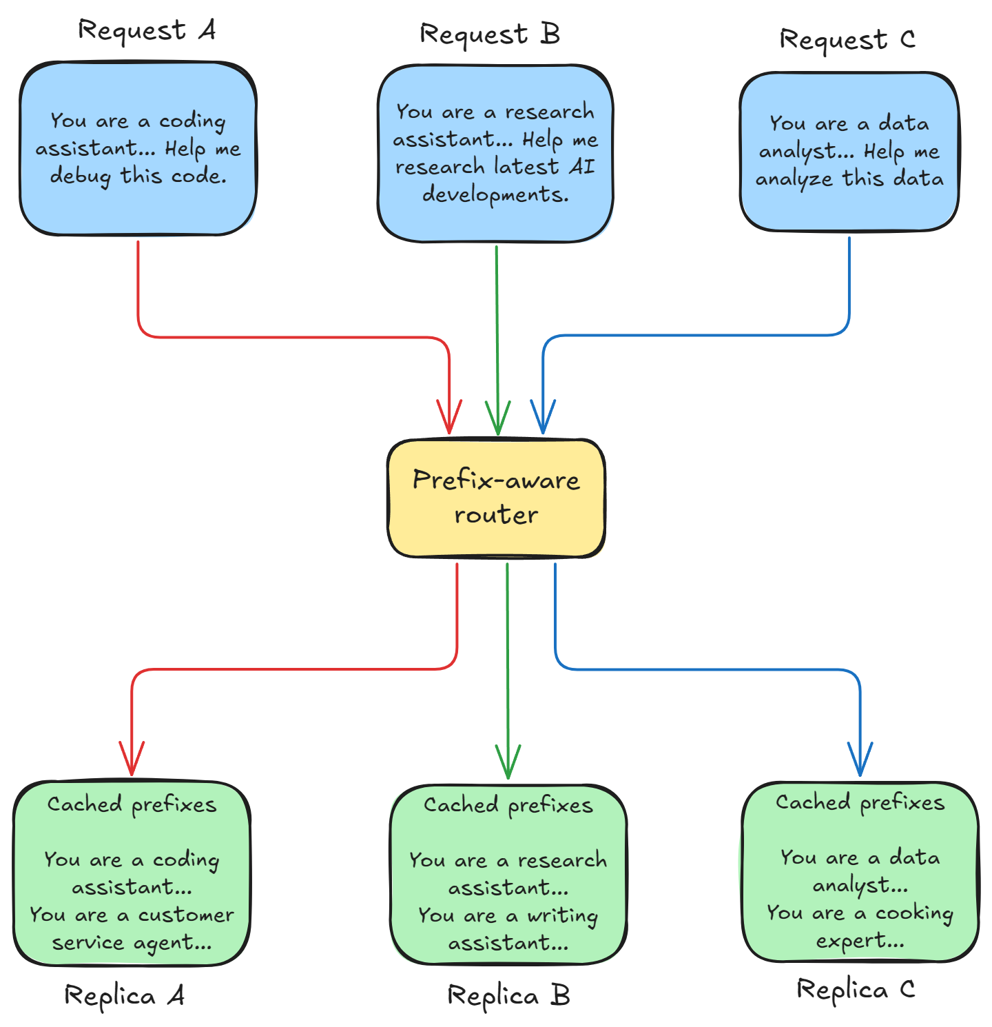
Different open-source frameworks each have their own implementations for prefix-aware routing.
Generally, prefix-aware routing requires the router to maintain a map or table (or use a predictive algorithm) that tracks which KV prefixes are currently cached on which GPU replicas.
When a new query arrives, the router sends the query to the replica that has the relevant prefix already cached.
Model sharding strategies
There are several strategies to scale a dense ML model (discussed here):

LLMs, like Mixture of Experts (MoE), are complicated.

MoE models use a specialized parallelism strategy called expert parallelism, which splits the experts themselves across different devices, and the attention layers are replicated across all GPUs:
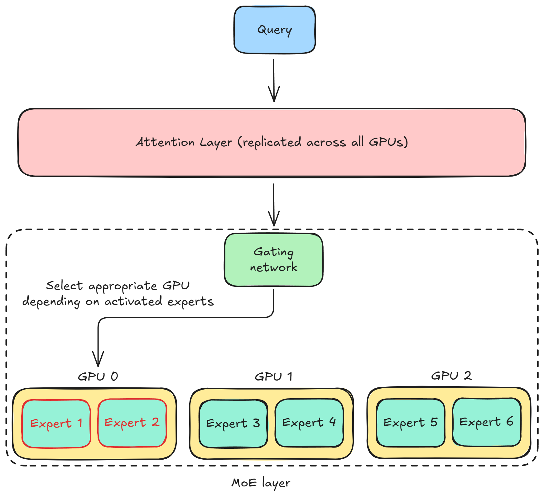
So each GPU holds the full weights of only some experts, not all. This means that each GPU processes only the tokens assigned to the experts stored on that GPU.
Now, when a query arrives, the gating network in the MoE layer dynamically decides which GPU it should go to, depending on which experts are activated.
This is a complex internal routing problem that cannot be treated like a simple replicated model. You need a sophisticated inference engine to manage the dynamic flow of computation across the sharded expert pool.
If you want to learn the full LLMOps lifecycle, we have covered every bit of it in the LLMOps course, starting from fundamentals to production:
Read Part 2 on understanding the core building blocks of LLMs →
Read Part 3 on the key components of LLMs, focusing on the attention mechanism, architectures like transformers and mixture-of-experts, and the fundamentals of pretraining and fine-tuning →
Read Part 4 on decoding strategies, generation parameters, best practices, and the broader lifecycle of LLM-based applications →
Read Part 5 on context + prompt engineering from a system perspective, in-context learning, types of prompts, and different prompting techniques →
Read Part 6 on prompt versioning, defensive prompting, and techniques like verbalized sampling, role prompting, and more →
Read Part 7 on context engineering, covering context types, context construction principles, and retrieval-centric techniques for building high-signal inputs →
Read Part 8 on memory, dynamic, and temporal context in LLM systems, covering short and long-term memory, dynamic context injection, and common failure modes in agentic applications →
Read Part 9 on evaluation methods and approaches for LLM-based applications, primarily focusing on building a strong understanding of the fundamental concepts →
Read Part 10 on evaluation benchmarks in LLM applications, with task-specific methodologies, and the core tooling for evaluation of LLM apps →
Read Part 11 on evaluation of multi-turn systems, tool use evaluations, tracing, and red teaming →
Read Part 12 on LLM fine-tuning, parameter-efficient methods like LoRA and QLoRA, and alignment techniques such as RLHF, DPO, and GRPO →
Read Part 13 on LLM inference optimization, KV caching, PagedAttention, FlashAttention, speculative decoding, and model parallelism →
Read Part 14 on the fundamentals of LLM serving, including API-based access, inference with vLLM, and practical decisions →
👉 Over to you: What are some other differences between LLM inference and regular inference?
Good day!