RAG & Fine-tuning in LLMs

...explained visually.

Free AI Skill Badges to learn production AI capabilities

MongoDB put together an AI Skill Badges program on MongoDB University with hands-on learning tracks for developers building production-grade AI applications.

Three standout AI Skill Badges you should start with:

1. Auto-embedding AI Models: Learn how to generate vector embeddings directly inside MongoDB without a separate embedding pipeline.

2. Agentic Memory with MongoDB: Design short and long-term memory for AI agents using MongoDB, LangGraph, vector search, and Voyage AI.

3. Voyage AI for Semantic Search and RAG: Build a two-step retrieval pipeline using Voyage AI and MongoDB’s auto-embedding to improve relevance while controlling latency and cost.

Beyond the three, MongoDB University also covers AI Skill Badges like:

↳ AI Data Strategy with MongoDB

↳ Building an App with Code Agents and MongoDB

↳ Vector Search Fundamentals

↳ RAG with MongoDB

↳ AI Agents with MongoDB

Every badge focuses on building working systems, not walkthroughs of abstract concepts.

Start learning for free here →

Thanks to MongoDB for making this public and partnering with us today.

---

RAG & Fine-tuning in LLMs

If you’re building real-world LLM apps, you can rarely use a model out of the box without adjustments.

Devs typically treat RAG and fine-tuning as interchangeable options, but in reality, they are not.

RAG and fine-tuning solve fundamentally different problems. One controls what the model knows at runtime. The other changes how the model behaves by default.

This visual breaks it down for you:

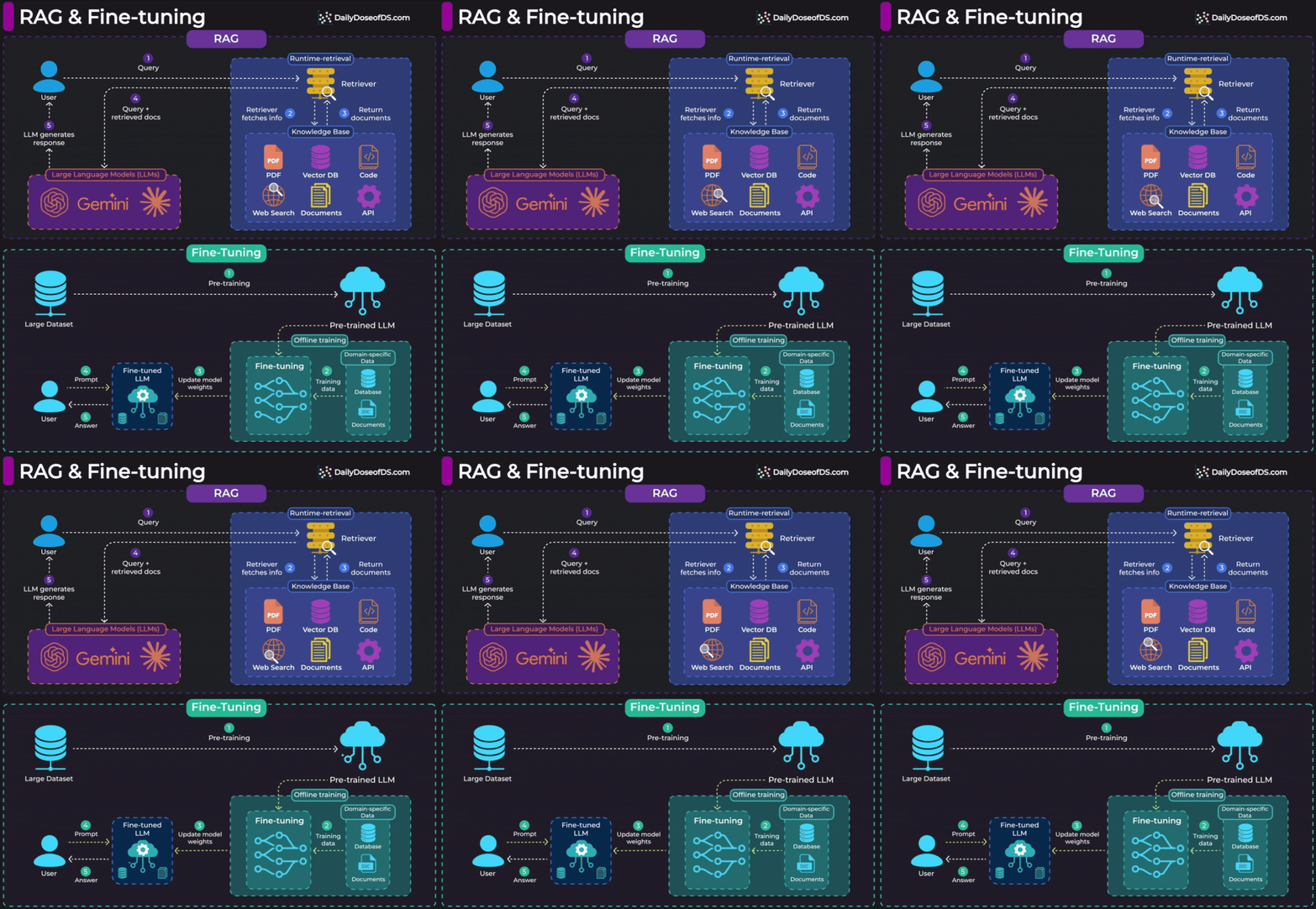
For RAG, look at the top half of the visual.

RAG operates at inference time. When a user sends a query, the retriever searches your knowledge base (PDFs, vector DBs, APIs, documents), pulls relevant context, and passes it to the LLM along with the query. The model weights never change. You’re giving the LLM a “cheat sheet” at runtime.

Fine-tuning is different. To understand, look at the bottom half of the visual.

It happens offline, before deployment. You train the model on domain-specific data, and the weights actually update. The model now behaves differently by default.

Fine-tuning is for changing how the model behaves. Its tone, vocabulary, response structure, or specialized reasoning patterns.

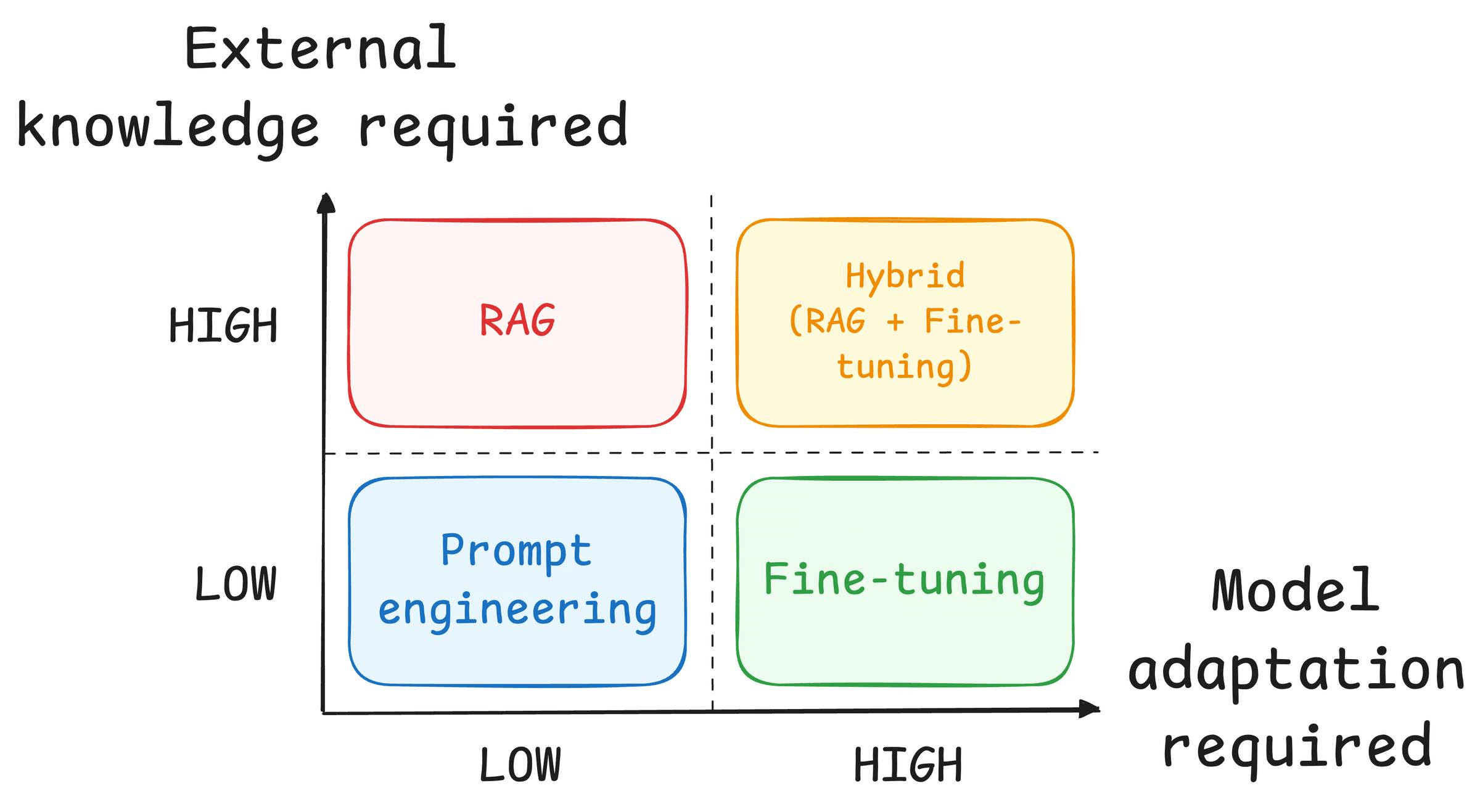
Two questions guide which one you need:

• How much external knowledge does your task require?

• How much behavioral adaptation do you need?

If you need the model to reference specific documents, product catalogs, or anything that updates frequently, that’s mostly a RAG territory.

If you need the model to adopt internal vocabulary, match a specific writing style, or follow domain-specific reasoning patterns, that’s mostly a fine-tuning territory.

For instance, an LLM might struggle to summarize company meeting transcripts because speakers use internal jargon the model has never seen. Fine-tuning fixes this.

That said, in production systems, you might often need both. A customer support bot might need to pull answers from documentation (RAG) while responding in your brand’s voice (fine-tuning).

The simple takeaway:

• RAG → What should the model know?

• Fine-tuning → How should the model behave

They’re not competing. They’re complementary layers in an LLM stack.

On a side note, we started a beginner-friendly crash course on RAGs recently with implementations, which covers:

• ​​RAG fundamentals​​​​​

• ​RAG evaluation​

• ​​​​​RAG optimization​​​​​

• ​Multimodal RAG​

• ​​​​​Graph RAG​​

• ​​Multivector retrieval using ColBERT​

• ​​​​​RAG over complex real-world docs ft. ColPali

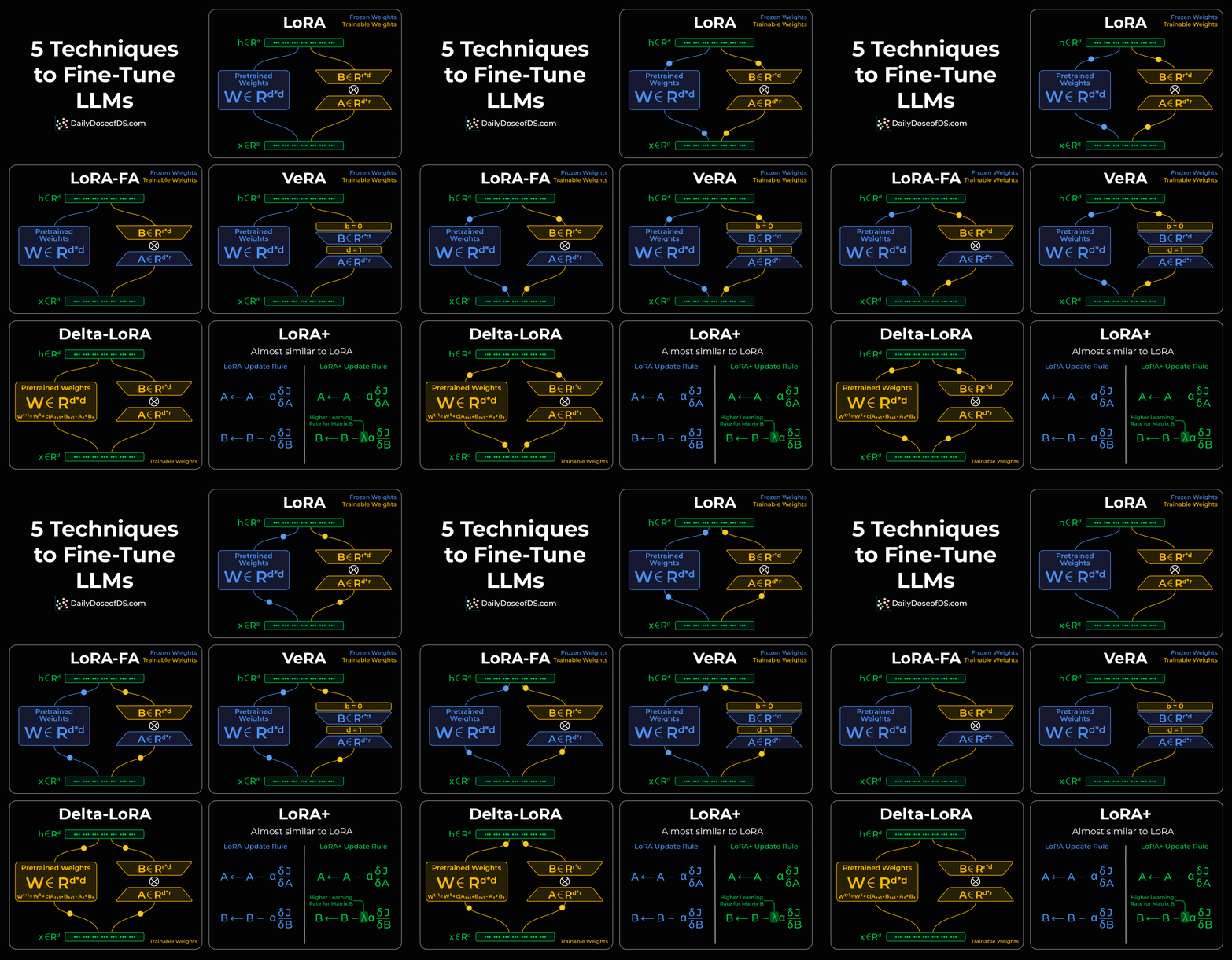
Also, we have covered several LLM fine-tuning with code techniques below:

• Understanding LoRA-derived Techniques for Optimal LLM Fine-tuning.

• Implementing LoRA From Scratch for Fine-tuning LLMs.

• Implementing DoRA (an Improved LoRA) from Scratch.

---

​ANN search using inverted file index​

kNN performs an exhaustive search, which is inefficient at scale!

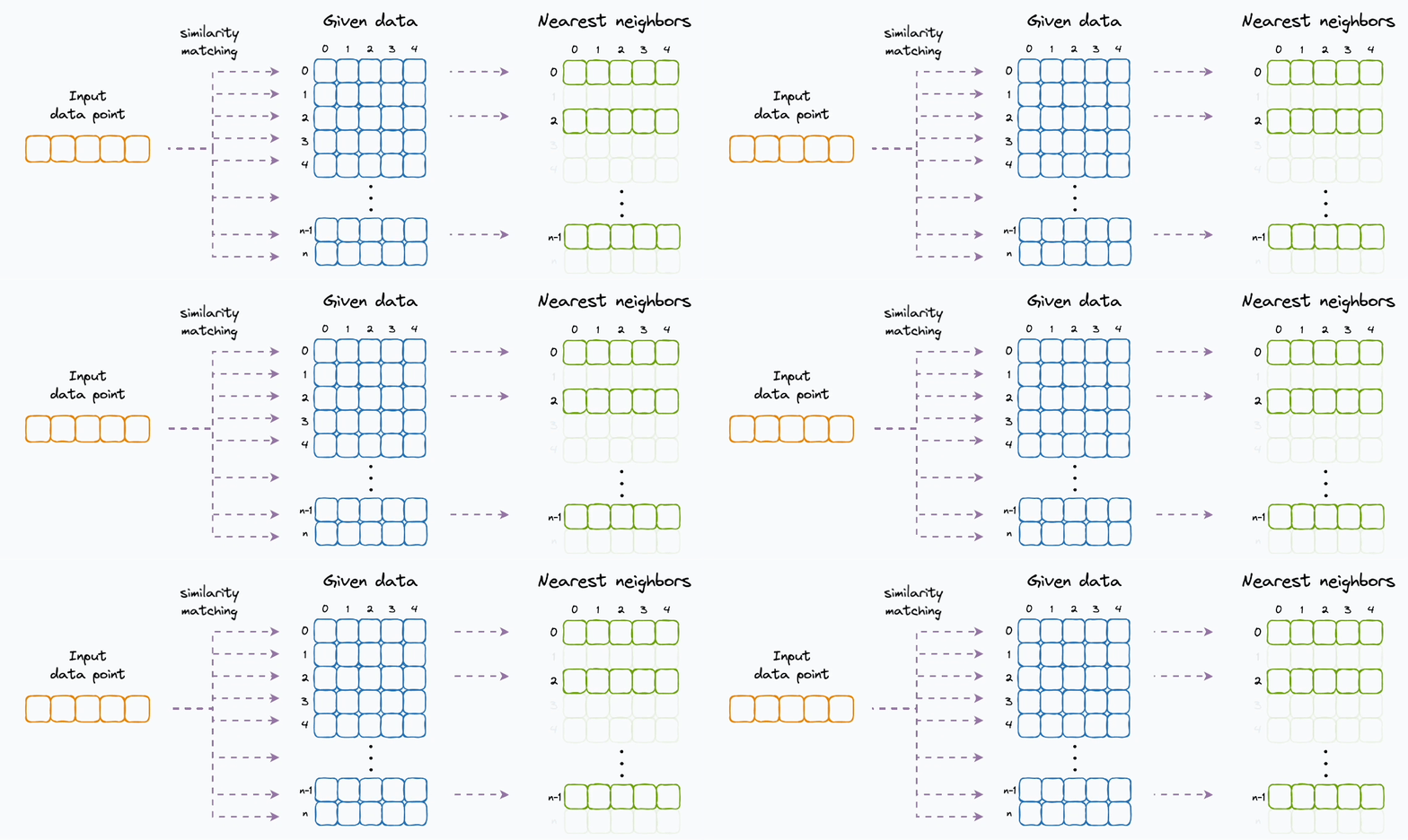
Approximate nearest neighbor search algorithms solve this.

The core idea is to narrow down the search space using indexing techniques, which improves the run-time performance.

Inverted file index (IFV) is one of the simplest and intuitive techniques to do this.

Steps for indexing:

• Partition the given data using techniques like k-means.

• Each partition gets a centroid, and each data point gets associated with only one partition.

• A map holds all the data points that belong to a centroid’s partition.

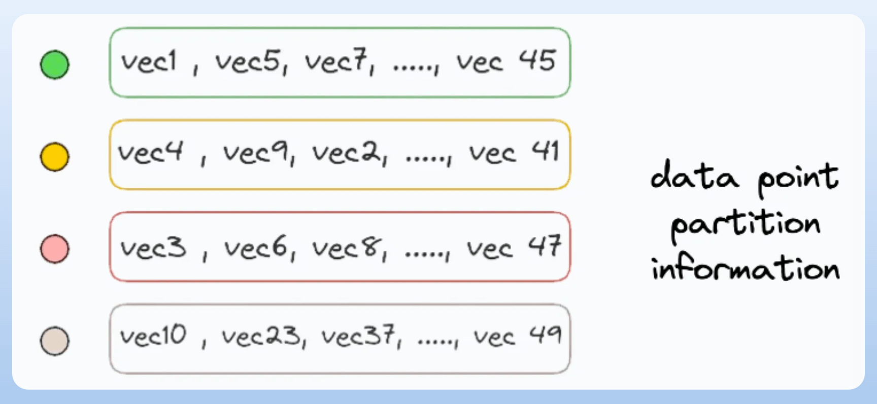
Indexing done!

Here’s how we search.

• First, find the closest centroid to the query:

• Next, find the nearest neighbor among only those data points that belong to the closest centroid’s partition:

This drastically reduces the run-time.

Consider:

• There are N data points.

• Each data point is D-dimensional.

• We create K partitions.

• Lastly, for simplicity, let’s assume that each partition gets equal data points.

In kNN, the query data point is matched to all N data points, which makes the time complexity → O(ND).

In IFV, however, there are two steps:

1. Match to all centroids → O(KD).

2. Find the nearest neighbor in the nearest partition → O(ND/K).

The final time complexity comes out to be the following:

…which is significantly lower than that of kNN.

Assume → N=10M and k=100:

• The search complexity of kNN will be proportional to 10M.

• With IFV, the search complexity will be proportional to 100 + 100k = 100100, which is nearly 100 times faster.

That said, ANN is not always accurate.

If some data points are actually close to the query data point but not in the same partition, they may still get missed:

We willingly accept such trade-offs to reduce latency.

In the deep dives on vector databases (open access), we discussed 4 such techniques, along with an entirely beginner-friendly and thorough discussion on Vector Databases.

Check it out here if you haven’t already: ​A Beginner-friendly and Comprehensive Deep Dive on Vector Databases.

Good day!