

In today’s newsletter:
Build voice agents that hear the details.
RAG vs. Jev + RAG, clearly explained!
5 vector DB indexing strategies.
Build voice agents that hear the details
Speechmatics Linden is a speech-to-text model built specifically for voice agents. It focuses on the inputs that tend to cause expensive mistakes: strong accents, background noise, non-native speech, names, and alphanumeric strings such as booking references.
Real-time transcription across 55+ languages
Final transcripts in roughly 250 ms after a
ForceEndOfUtterancesignalCustom dictionaries for names, product terms, and industry vocabulary
Native integrations for LiveKit, Pipecat, Jambonz, and the Speechmatics API
Linden 1 costs $0.30 per hour for new users, with volume discounts bringing the price down to $0.16 per hour
New accounts receive $100 in credit with no card required, which covers roughly 333 hours of Linden 1 transcription at the standard $0.30 per-hour rate.
Thanks to Speechmatics for partnering today!
RAG vs. Jev + RAG, clearly explained!
In a standard RAG setup, documents are split into chunks, converted into embeddings, and stored in a vector DB.
When a query arrives, the system embeds it and retrieves the top-k chunks with the closest vectors.
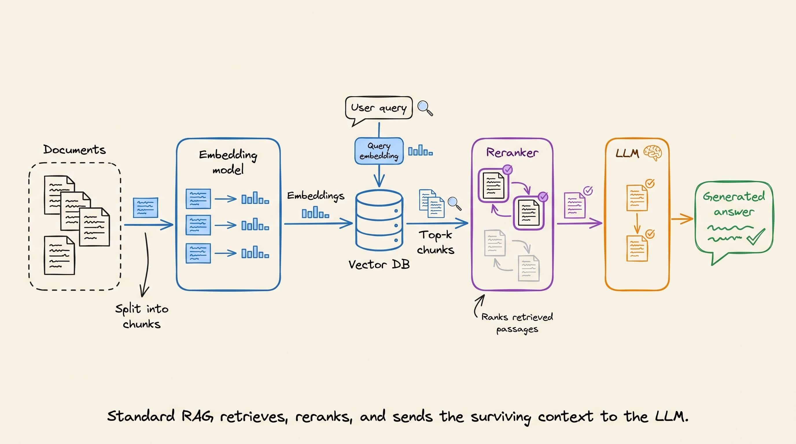
Many production setups add a reranker after retrieval.
The reranker compares the query with each retrieved passage, improves their ordering, and keeps the highest-scoring results.
Those passages are then placed in the context window, and the LLM generates an answer from them.
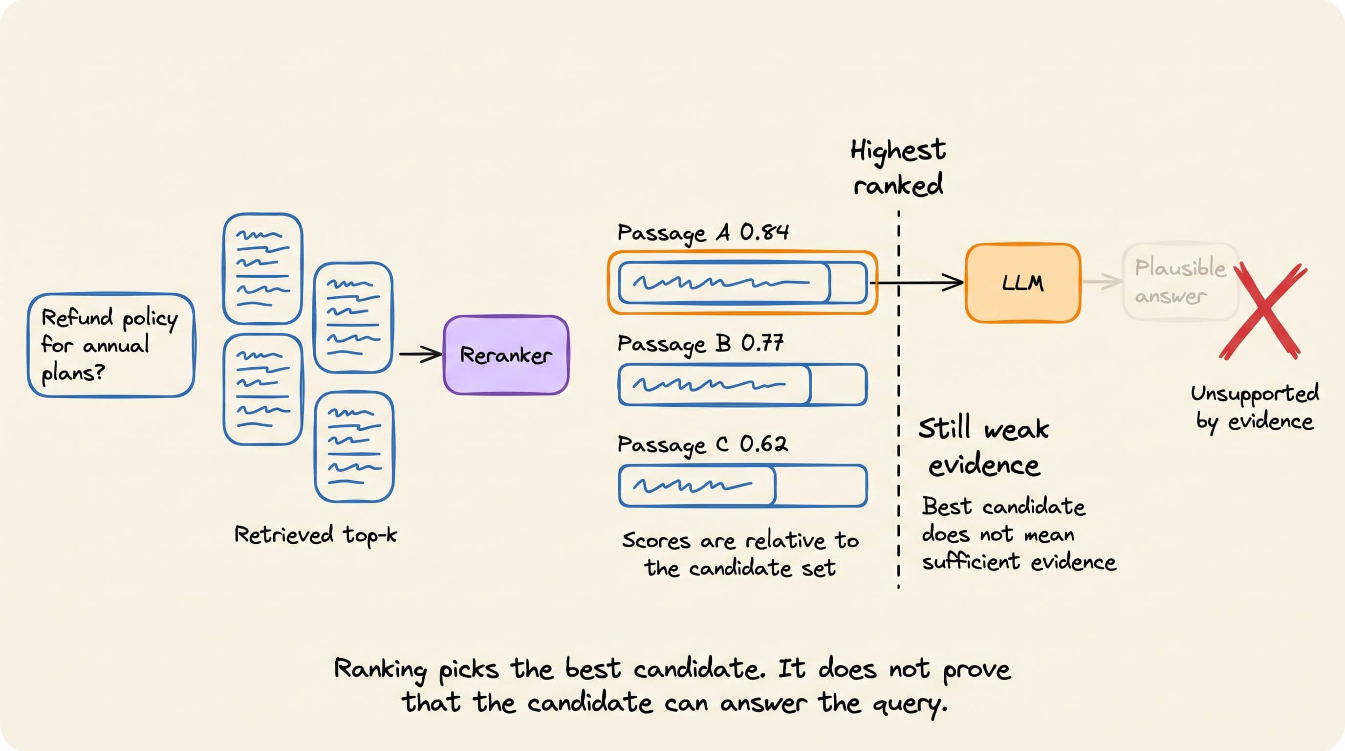
The problem is that ranking and answerability are different questions.
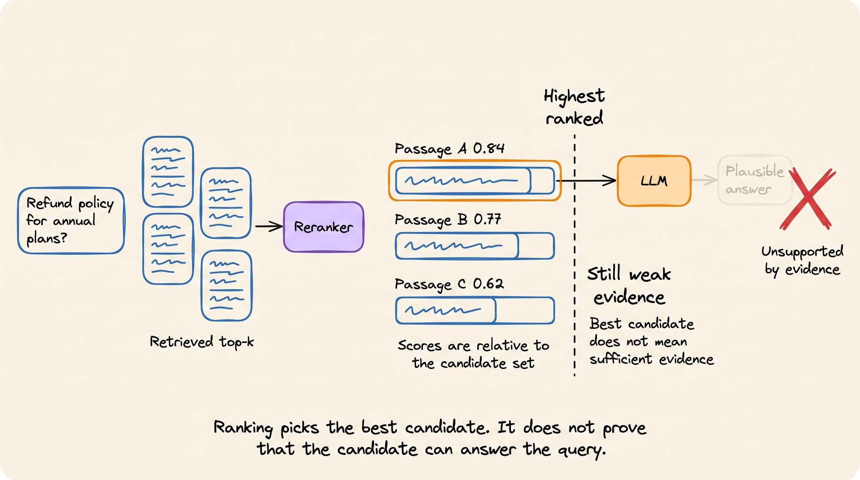
A passage can be more relevant than the other candidates while still containing weak, incomplete, or merely adjacent evidence.
The LLM receives it anyway and may produce a plausible answer from context that never supported one.
Jev + RAG keeps the retrieval stage as is but changes what happens before generation.
Instead of using a conventional reranker at this stage, Jev can judge every retrieved candidate against a typed question such as:
“Does this passage help answer the query?”
The query becomes the shared state, while the retrieved passages become individual candidates. Jev evaluates them together and returns a probability for each one.
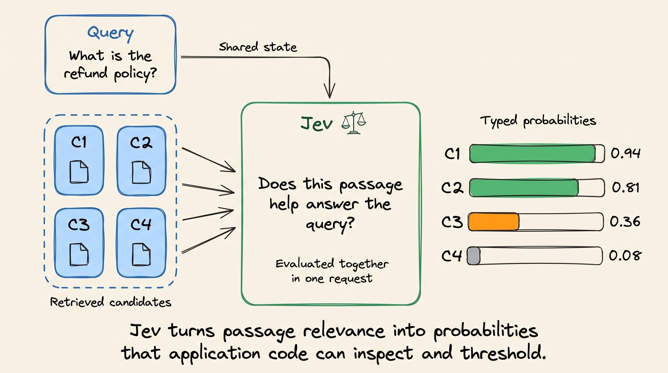
Application code then applies a threshold.
↳ Candidates above the threshold continue to the LLM.
↳ Candidates below it are removed from the context window.
The same Jev request can also judge whether the remaining evidence is sufficient to answer the query.
If answerability falls below the threshold, the application can skip the LLM and return “not in the documents.”
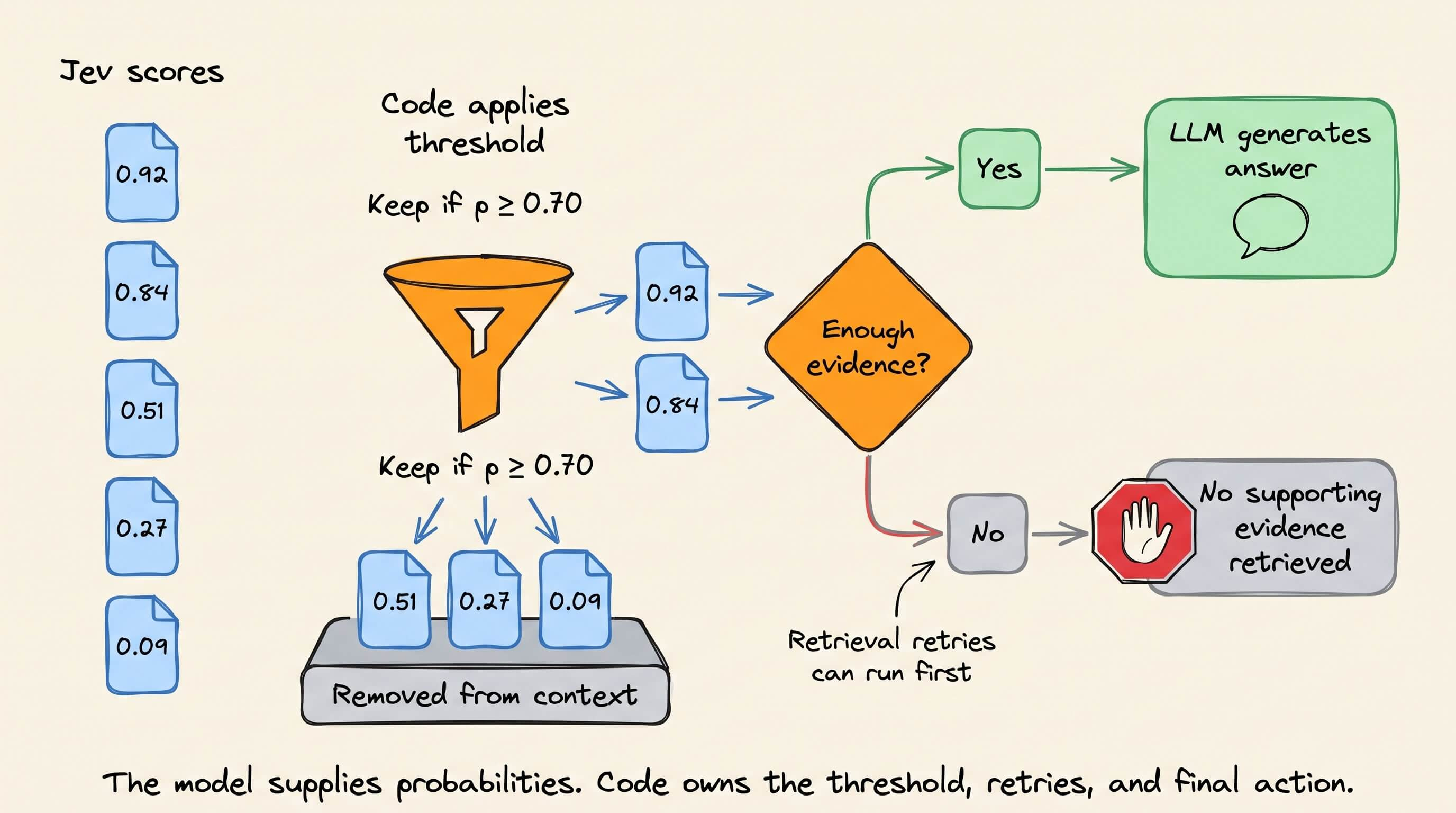
Jev does not replace the embedding model, vector database, or generation model. Retrieval still sets the cap because Jev cannot recover a passage that never entered the candidate set.
The diagram below depicts the complete flow.
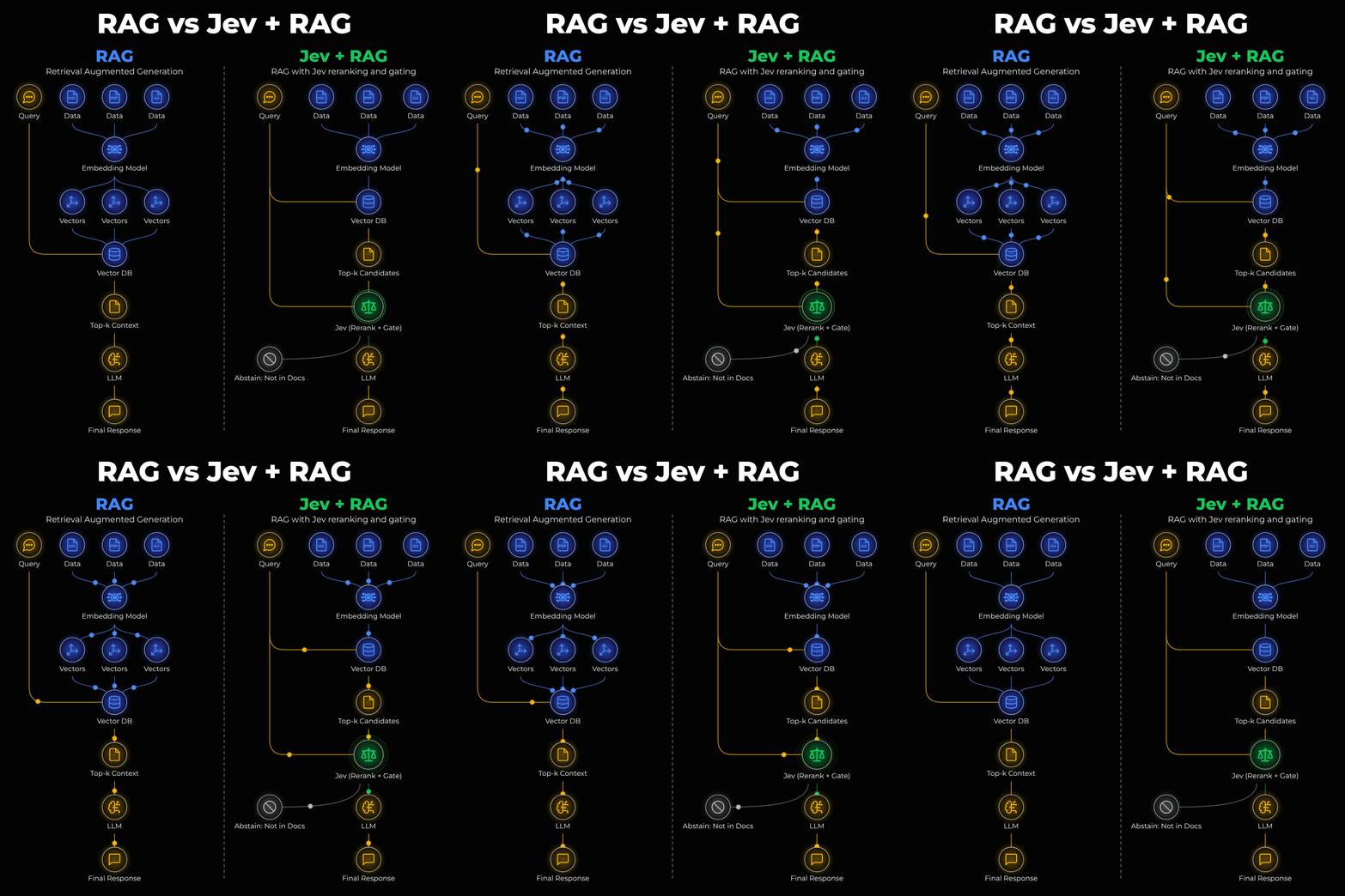
RAG retrieves a broad candidate set.
Jev reranks and gates those candidates.
The LLM generates an answer.
Jev becomes more useful when the same typed decisions sit inside a complete agent loop. Parts 3 and 4 of our Agent Engineering course implement that system end to end:
Part 3: Build routing, guardrails, and approval controls with LangGraph and Jev →
Part 4: Add planning, verification, replanning, and stopping logic →
5 vector DB indexing strategies
Meta. Google. Microsoft.
These companies have spent years engineering faster vector-search systems.
A basic nearest-neighbor query computes the distance between the query and every stored vector.
Its cost grows linearly with the size of the database and becomes impractical across millions of candidates.
Every vector index reduces this computation differently, using clustering, graph traversal, compression, or a combination of these methods.
Here are five common approaches:
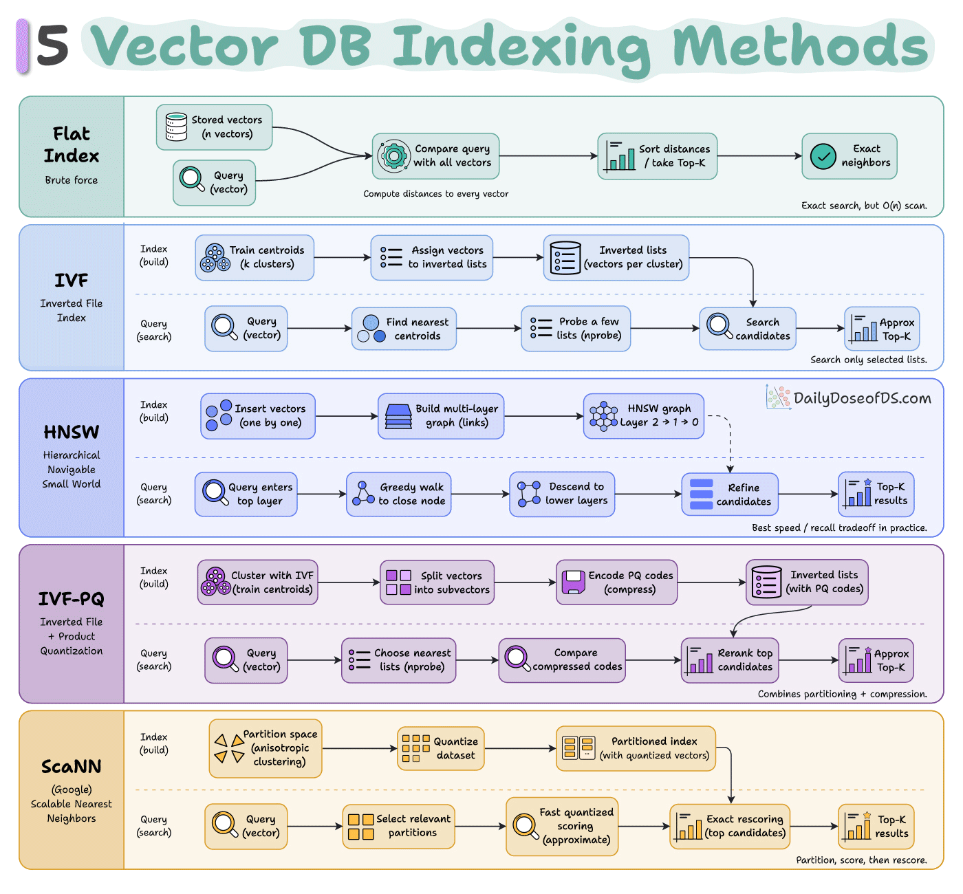
This full article covers the first four techniques in detail, with an architectural breakdown →
1. Flat index
A Flat index compares the query with every stored vector, selects the K smallest distances, and returns them.
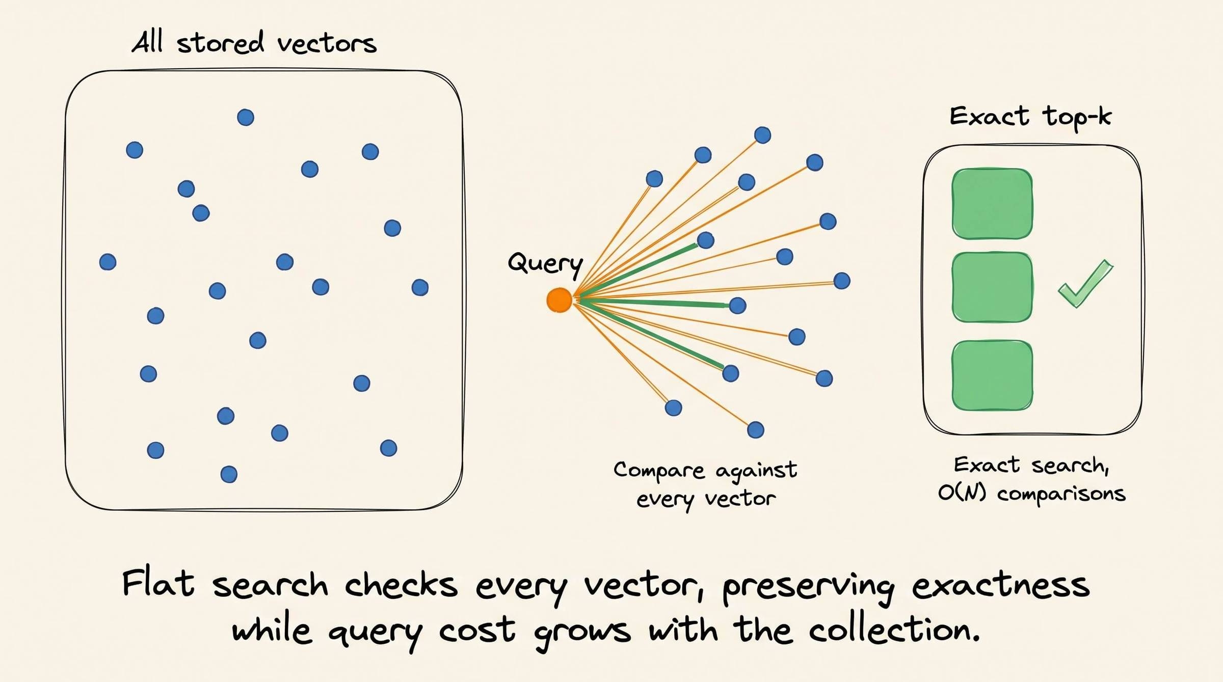
It performs an exact search, so it is useful when accuracy matters and the dataset is small enough to scan.
The query cost grows linearly with the number of stored vectors.
2. IVF
IVF divides the vector space into clusters. Each stored vector is assigned to its nearest cluster centroid.
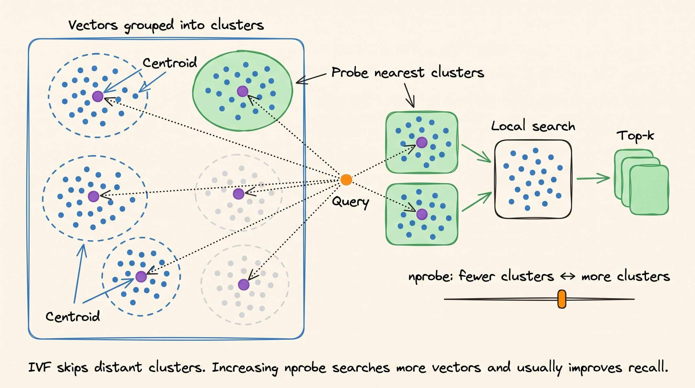
At query time, the database finds the closest centroids and searches only their clusters.
A probe parameter controls how many clusters it searches, and increasing it usually improves recall but also increases latency.
3. HNSW
HNSW stores vectors in a multilayer graph.
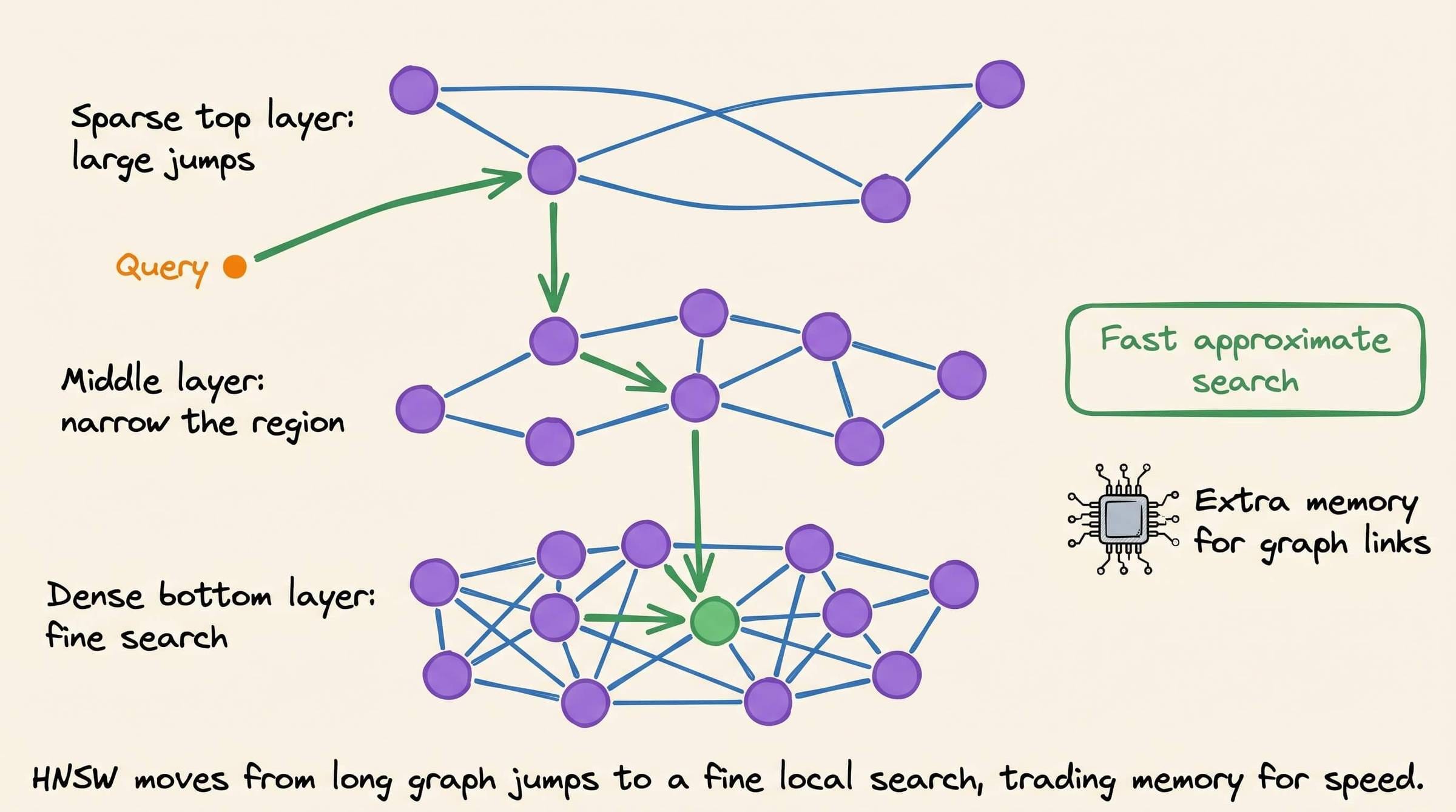
The upper layers contain fewer nodes and allow large jumps through the graph. Lower layers contain more nodes and support a finer search.
A query starts at the top, moves toward closer nodes, and descends through the layers. HNSW often provides low latency and high recall, but the graph requires extra memory.
4. IVF-PQ
IVF-PQ combines clustering with product quantization.
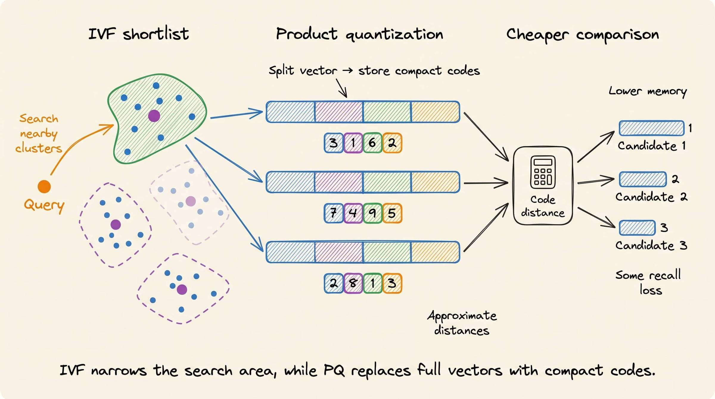
IVF limits the search to a few relevant clusters. Product quantization splits each vector into smaller parts and stores compact codes for them.
Comparing these codes is cheaper than comparing full-precision vectors. This reduces memory use and query cost, with some loss in recall.
5. ScaNN
ScaNN partitions the dataset and stores quantized vector representations.
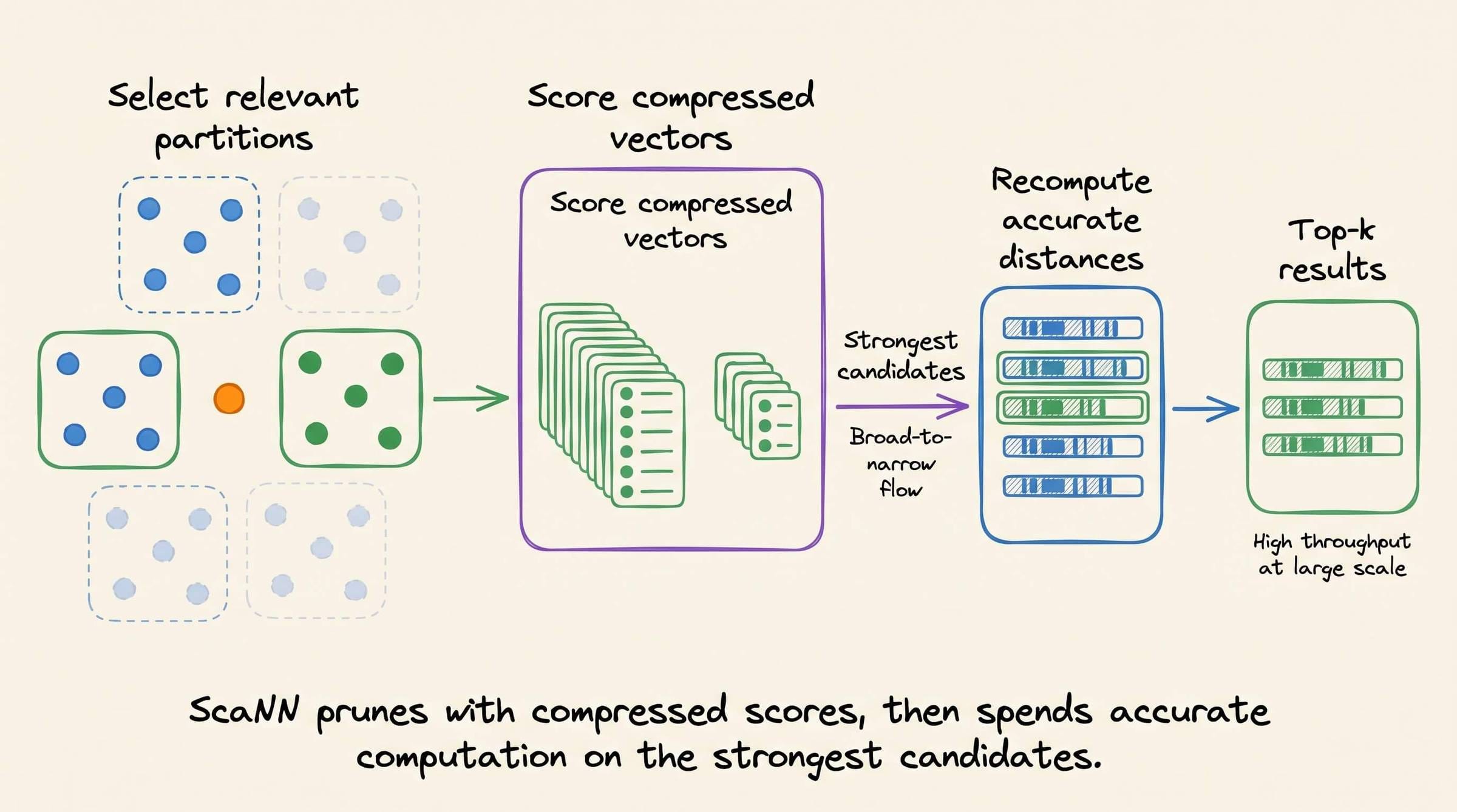
During search, it selects relevant partitions, scores compressed candidates, and recalculates more accurate distances for the strongest candidates.
This makes it suitable for large datasets where throughput matters.
The choice depends on the system constraints.
Flat prioritizes exact results.
HNSW trades memory for speed.
IVF provides direct control over the amount of search work.
IVF-PQ and ScaNN reduce the memory and compute required for large collections.
Choosing an index requires deciding what your system can afford to trade.
Index selection is one part of building a production RAG system. Our 15-part RAG Systems course develops the rest of the stack progressively:
Part 1: Build the complete RAG workflow, including chunking, embeddings, retrieval, and reranking →
Part 2: Evaluate retrieval and generation quality with RAG-specific metrics →
Part 3: Reduce RAG latency with faster retrieval and generation paths →
Part 5: Understand CLIP embeddings, multimodal prompting, and tool calling →
Part 6: Build a multimodal RAG system over real-world data →
Part 7: Use Graph RAG for relationships that ordinary chunk retrieval misses →
Part 10: Apply the first set of techniques for production RAG systems →
Part 11: Complete the production RAG techniques and implementation patterns →
Part 12: Reduce prefill latency by reusing KV caches without a shared prefix →
Part 13: Preload a corpus before queries arrive and examine the production constraints →
Part 14: Compress preloaded caches and measure where the approaches break →
Part 15: Implement Block-Attention, Cartridges, and production preloading →
Good day!