Reduce Trees in Random Forest Model

The coolest trick to improve random forest models.

Daily Dose of Data Science Free Book | Deep Dives

I use random forests quite often, and I have consistently noticed that we always create many more decision trees than required.

Of course, this can be tuned as a hyperparameter, but it requires training many different random forest models, which takes time.

Today, I will share one of the most incredible tricks I formulated recently to:

• Increase the accuracy of a random forest model

• Decrease its size.

• Drastically increase its prediction run-time.

And all this without having to ever retrain the model.

Let’s begin!

---

Logic

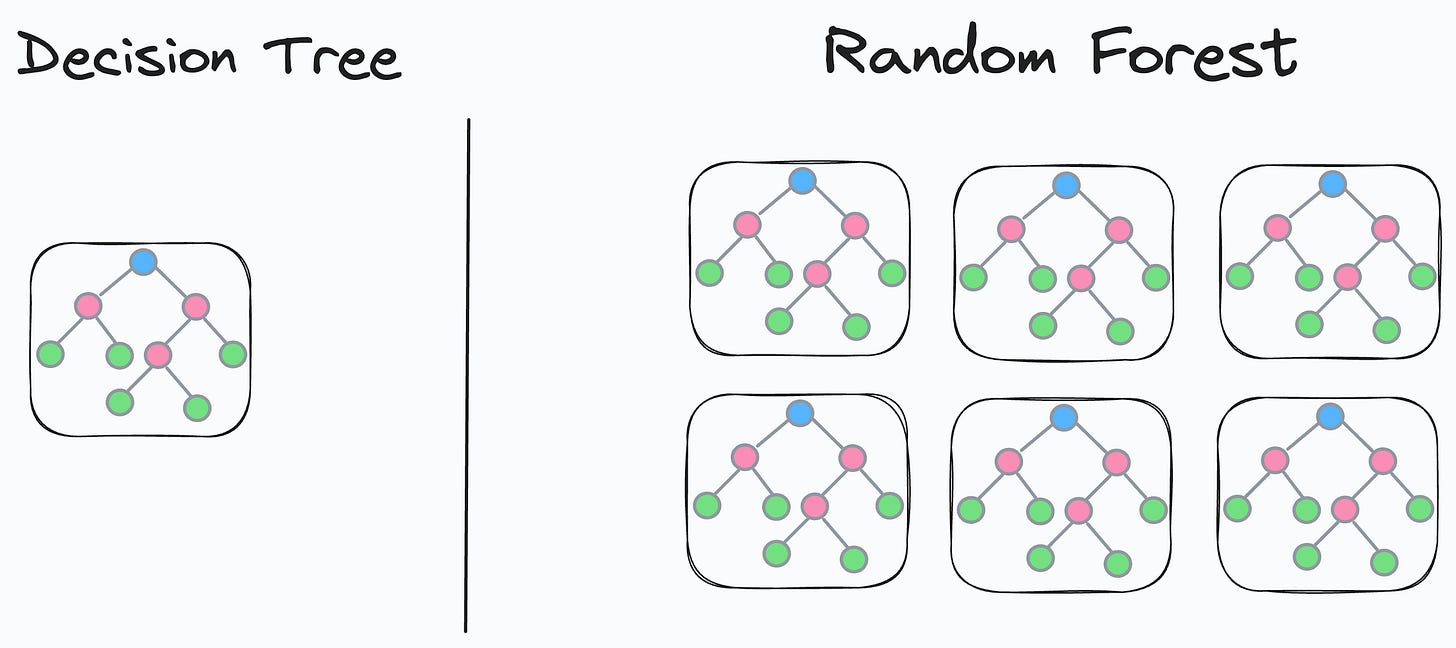
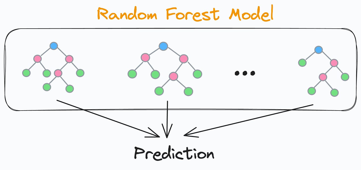
We know that a random forest model is an ensemble of many different decision trees:

The final prediction is generated by aggregating the predictions from each individual and independent decision tree.

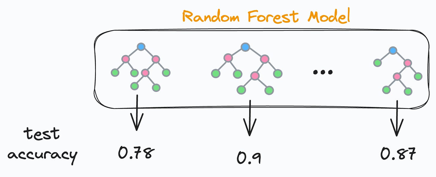
As each decision tree in a random forest is independent, this means that each decision tree will have some validation accuracy, right?

This also means there will be some underperforming and some well-performing decision trees. Agreed?

So what if we do the following:

• We find the validation accuracy of every decision tree.

• We sort the accuracies in decreasing order.

• We keep only the “k” top-performing decision trees and remove the rest.

Once done, we’ll be only left with the best-performing decision trees in our random forest, as evaluated on the validation set.

Cool, isn’t it?

---

Now, how to decide “k”?

It’s simple.

We can create a cumulative accuracy plot.

It will be a line plot depicting the accuracy of the random forest:

• Considering only the first two decision trees.

• Considering only the first three decision trees.

• Considering only the first four decision trees.

• And so on.

It is expected that the accuracy will first increase with the number of decision trees and then decrease.

Looking at this plot, we can find the most optimal “k.”

---

Implementation

Let’s look at its implementation.

First, we train our random forest as we usually would:

Train the RF model

Next, we must compute the accuracy of each decision tree model.

In sklearn, individual trees can be accessed with model.estimators_ attribute.

Estimators of random forest are a list of decision trees

Thus, we iterate over all trees and compute their validation accuracy:

Compute the accuracy of all trees

The model_accs is a NumPy array that stores tree id and its validation accuracy:

>>> model_accs
array([[ 0.   ,  0.815], # [tree id, validation accuracy]
       [ 1.   ,  0.77 ],
       [ 2.   ,  0.795],
          ...

Now, we must rearrange the decision tree models in the model.estimators_ list in decreasing order of validation accuracies:

# sort on second column in reverse order to obtain sorting order
>>> sorted_indices = np.argsort(model_accs[:, 1])[::-1]

# obtain list of model ids according to sorted model accuracies
>>> model_ids = model_accs[sorted_indices][:,0].astype(int)
array([65, 97, 18, 24, 38, 11,...

This list tells us that the 65th indexed model is the highest performing, followed by 97th indexed, and so on….

Now, let’s rearrange the tree models in model.estimators_ list in the order of model_ids:

# create numpy array, rearrange the models and convert back to list
model.estimators_ = np.array(model.estimators_)[model_ids].tolist()

Done!

Finally, we create the plot discussed earlier.

It will be a line plot depicting the accuracy of the random forest:

• By considering only the first two decision trees.

• By considering only the first three decision trees.

• By considering only the first four decision trees.

• and so on.

The code to compute cumulative accuracies is demonstrated below:

Create the cumulative accuracy plot

In the above code:

• We create a copy of the base model called small_model.

• In each iteration, we set small_model’s trees to the first “k” trees of the base model.

• Finally, we score the small_model with just “k” trees.

Plotting the cumulative accuracy result, we get the following plot:

Cumulative accuracy score

It is clear that the max validation accuracy appears by only considering 10 trees, which is a ten-fold reduction in the number of trees.

Comparing their accuracy and run-time, we get:

• We get a 6.5% accuracy boost.

• 13 times prediction faster run-time.

Now, tell me something:

• Did we do any retraining or hyperparameter tuning? No.

• As we reduced the number of decision trees, didn’t we improve the run time? Of course, we did.

Isn’t that cool?

Of course, one thing to note here is that it is not recommended to overly reduce the ensemble size because we want to ensure our RF still maintains many different types of decision trees.

Also, try not to overfit the validation set by selecting only those trees that perform the best on the validation set.

Instead, the approach to selecting the best k will often be quite subjective and it does not necessarily have to rely solely on the validation accuracy but could be based on various factors.

What are your thoughts?

If you are always curious about the mathematical details and wish to dive into Bagging (from a mathematical angle), we covered it here: Why Bagging is So Ridiculously Effective At Variance Reduction?

It covers every little detail that will uncover:

1. Why Bagging is so effective?

2. Why do we sample rows from the training dataset with replacement?

3. How to mathematically formulate the idea of Bagging and prove variance reduction?

You can download the notebook for today’s issue here: Jupyter Notebook

👉 Over to you: What are some other cool ways to improve model run-time?

---

Are you overwhelmed with the amount of information in ML/DS?

Every week, I publish no-fluff deep dives on topics that truly matter to your skills for ML/DS roles.

For instance:

• A Crash Course of Model Calibration – Part 1

• Conformal Predictions: Build Confidence in Your ML Model’s Predictions

• Quantization: Optimize ML Models to Run Them on Tiny Hardware

• A Crash Course on Causality – Part 1

• A Crash Course on Causality – Part 2

• A Beginner-friendly Introduction to Kolmogorov Arnold Networks (KANs)

• 5 Must-Know Ways to Test ML Models in Production (Implementation Included)

• A Beginner-Friendly Guide to Multi-GPU Model Training

• 8 Fatal (Yet Non-obvious) Pitfalls and Cautionary Measures in Data Science

• Implementing Parallelized CUDA Programs From Scratch Using CUDA Programming

• You Are Probably Building Inconsistent Classification Models Without Even Realizing

• And many many more.

Join below to unlock all full articles:

---

SPONSOR US

Get your product in front of 84,000 data scientists and other tech professionals.

Our newsletter puts your products and services directly in front of an audience that matters — thousands of leaders, senior data scientists, machine learning engineers, data analysts, etc., who have influence over significant tech decisions and big purchases.

To ensure your product reaches this influential audience, reserve your space here or reply to this email to ensure your product reaches this influential audience.