

Kimi K3 vs Opus 4.8 vs Fable 5 vs GPT-5.6 Sol

When Claude Opus 4.8 shipped on May 28, it was the most capable model available to the public.
Yesterday, Moonshot AI released Kimi K3, and it beats Opus 4.8 at max effort on four of five major benchmarks: BrowseComp, DeepSWE, GPQA Diamond, FrontierSWE, and HLE with tools.
And this is not just an Opus story. K3 matches Claude Fable 5 and GPT-5.6 Sol on several benchmarks and beats them on some, while its API is priced at roughly a third of Fable 5’s.
K3 is open weights. Moonshot says it will ship all 2.8 trillion parameters on July 27, which would make it the largest open model released so far.
Every closed frontier model is rented intelligence, accessed through an API the provider can reprice, deprecate, or shut off.
Last month proved why rented intelligence comes with risks. A US export directive forced Anthropic to take Fable 5 offline globally for 18 days.
Weights on a disk don’t have that failure mode since they run on private infrastructure, fine-tune on private data, and cannot be switched off by anyone.
Do note that the weights aren’t public yet, so until July 27, this is an API model like any other.
RLHF vs. DPO vs. GRPO in RL
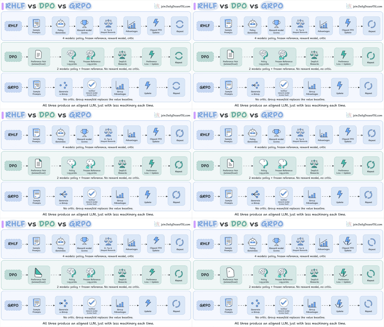
RLHF, DPO and GRPO are often grouped together as variations of the same algorithm.
But they take completely different approaches to teaching a model to behave the way you want, and those differences show up in the training setup, the data you need, and what it costs you at scale.
The visual below summarizes how they work:
Let’s understand this in detail today!
To dive deeper into these topics (with hands-on implementation and understand actual production tradeoffs), we have already covered every bit of it in the Reinforcement Learning Nanodegree:
RLHF (Reinforcement Learning from Human Feedback) is the simplest formulation, which also went into building ChatGPT.
You sample prompts, run them through the policy, and score the outputs with a reward model. Then you compute advantages, apply a KL penalty to keep the policy close to the reference, and update via PPO.
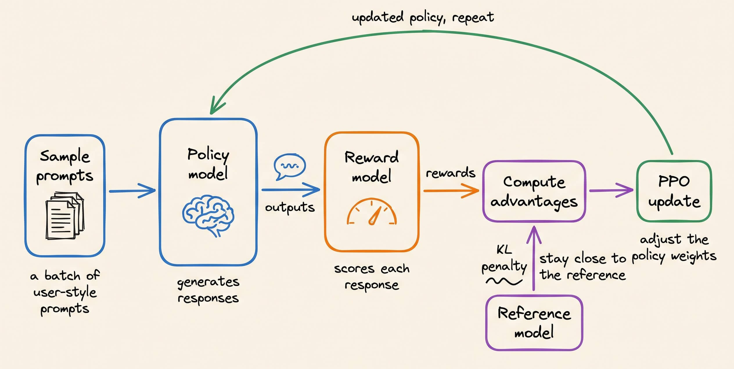
This requires four live models running simultaneously:
The policy you’re training
A frozen reference copy
A reward model
And a critic.
This means running four sets of forward passes per training step.
At production scale, this is expensive to run and hard to stabilize. And the reward model needs its own human-preference training before any of this can even begin.
DPO (Direct Preference Optimization) provides a better solution.
Instead of training a separate reward model, DPO derives the reward signal implicitly from the policy itself.
It works from preference pairs, a winner and a loser response to the same prompt. It computes log-probability ratios between the current policy and a frozen reference, and uses that ratio as the implicit reward.
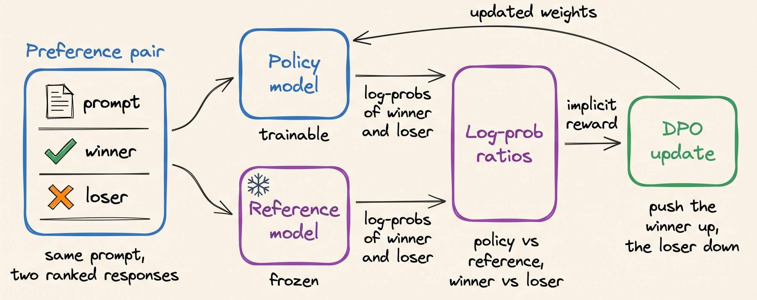
This removes the explicit reward model and the critic entirely, bringing the pipeline down to just policy and frozen reference.
The tradeoff is that you need labeled preference pairs upfront. And since there’s no online exploration, DPO can be brittle if the preference data doesn’t cover the failure modes you care about.
GRPO (Group Relative Policy Optimization), introduced by DeepSeek in 2024, takes a different path.
It keeps the RL framing but eliminates the critic by replacing the value baseline with group statistics.
For each prompt, the model generates a group of outputs, and a verifier scores each one. Advantages are then computed from the mean and standard deviation of those scores within the group.
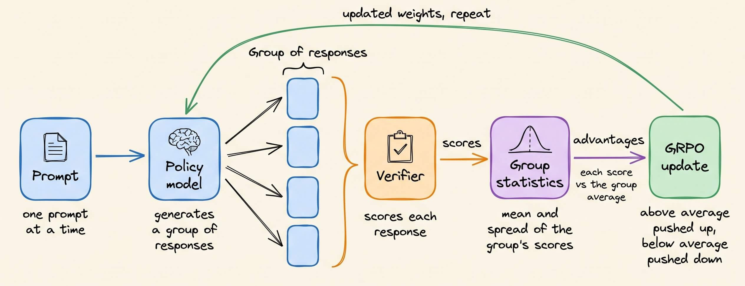
The critic is a key bottleneck in RLHF since it’s slow to converge, adds instability, and requires a regression head on top of the policy.
GRPO removes all of that by using the group itself as the baseline, keeping the RL loop intact but at lower overhead than PPO.
Here’s a useful way to understand all three at once.
RLHF uses external scores and an internal critic to measure advantage.
DPO encodes preference implicitly and skips both.
GRPO generates its own baseline from a group and keeps the RL loop without the critic.
All three produce aligned models, but they differ on how much machinery the alignment requires.
Paged Attention in LLMs
When you’re serving LLMs at scale, memory becomes your bottleneck before compute does.
The problem isn’t a lack of GPU memory; it’s how inefficiently we use it.
Let’s understand why this happens and how Paged Attention solves it elegantly!
KV Cache
During LLM inference, the model stores the key and value vectors of all previously generated tokens in memory. This is the KV cache (we covered KV caching in detail here).
Simply put, instead of recomputing attention over all previous tokens every time a new token is generated, the model just looks up the cached values and computes attention with them.
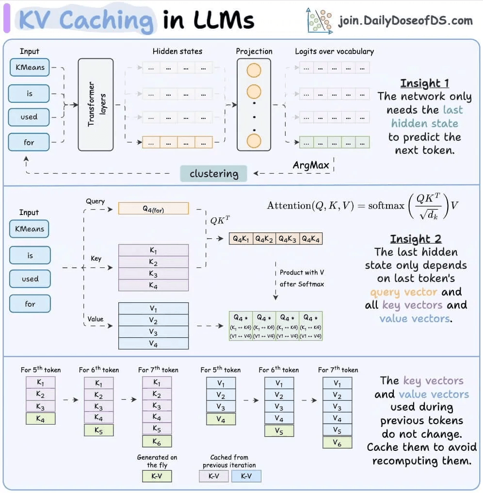
This is crucial for efficiency. Without it, generating a 1000-token response would require recomputing attention for all previous tokens at each step. That’s O(n²) operations instead of O(n) and the speed difference is evident below:
But there’s a problem.
The memory inefficiency problem
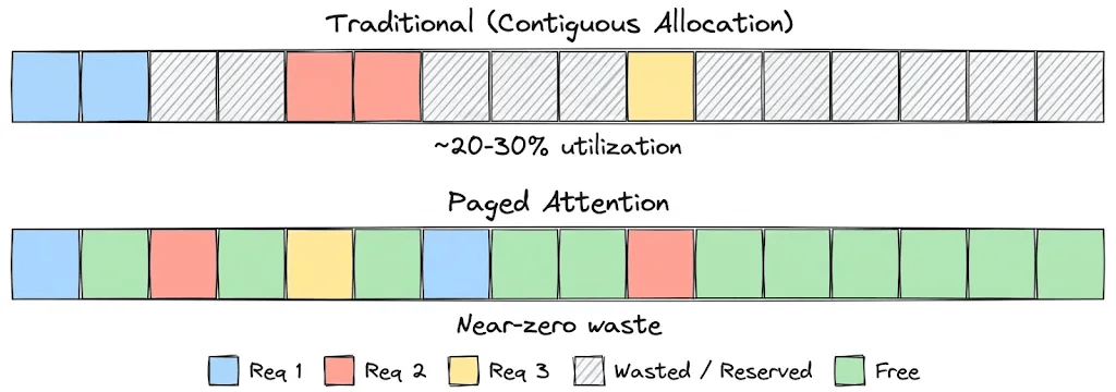
Traditional KV cache implementations pre-allocate large, contiguous memory blocks for each request.
Here’s why this is wasteful:
Imagine serving 100 concurrent users. You don’t know how long each response will be, so you pre-allocate space for the maximum possible length, say, 2048 tokens per request. But the average response turns out to be only 200 tokens.
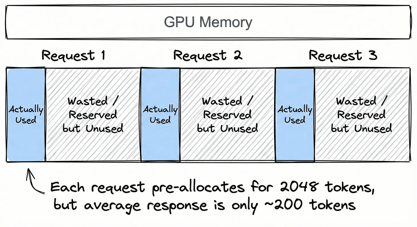
You’ve just reserved 10x the memory you actually need.
And it gets worse. Each request gets its own isolated block. So even if 80 of those 100 users share the same system prompt, you’re storing 80 duplicate copies of the same KV cache entries. None of that memory can be shared or reclaimed.
As a result, you’re often using only 20-30% of your allocated GPU memory effectively. The rest is reserved but unused, and because it’s scattered across fragmented contiguous blocks, you can’t even fit new requests into the gaps.
This is the core inefficiency that kills throughput.
Paged Attention
Paged Attention solves this by borrowing the concept of virtual paging memory from operating systems.
If you’ve studied OS fundamentals, you know that programs don’t get one big contiguous chunk of RAM. Instead, the OS breaks memory into small, fixed-size pages, scatters them anywhere in physical memory, and uses a page table to map each program’s virtual addresses to physical locations.
Paged Attention does the same thing for the KV cache. Here’s how:
Block-level allocation: Instead of reserving one large contiguous block per request, the KV cache is divided into small, fixed-size blocks (typically 16 tokens each). These blocks can live anywhere in GPU memory and don’t necessarily need to be next to each other.
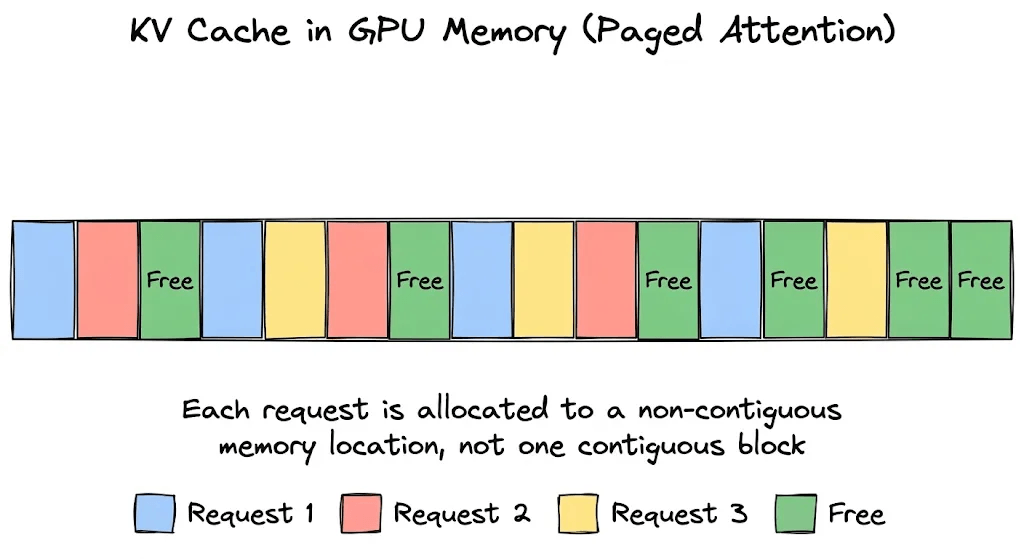
Block table (page table): Each request maintains a block table which is a simple mapping from logical block index to physical block location in GPU memory. When the model needs the KV cache for token 33, it looks up which physical block holds it, fetches it, and computes attention. The LLM doesn’t care where the block is physically sitting.
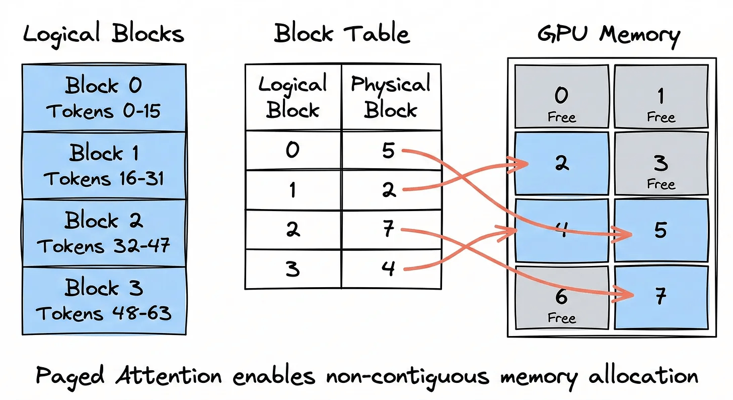
Shared prefixes: Here’s where it gets really clever. Multiple requests that share the same system prompt don’t need separate copies of the KV cache for that shared prefix. Their block tables simply point to the same physical blocks. Only when their responses diverge do new blocks get allocated for each request individually.
In a production setting, where every request typically shares a system prompt, the memory savings via shared prefix become massive.
Impact
In the original Paged Attention paper, the authors measured that existing systems only utilized 20-38% of the allocated KV cache memory effectively. The rest was wasted due to fragmentation and over-reservation.
Paged Attention can achieve:
2-4x higher throughput compared to state-of-the-art systems at the same level of latency
Near-zero memory waste, as it only allocates memory for what’s actually used
Better batching leads to more concurrent requests on the same GPU hardware
This is why vLLM, which implements Paged Attention as its core algorithm, has become the go-to inference engine for production deployments. Other frameworks like TensorRT-LLM and SGLang have also adopted similar paging mechanisms for faster inference.
This optimization becomes even more crucial when running inference servers at scale, especially with variable request patterns, shared prompts, and cost-per-request constraints.
👉 Over to you: What other OS concepts do you think could be applied to optimize LLM inference?
To dive deeper into how LLM systems are deployed, start with the practical and hands-on LLMOps course here →
Good day!