
SNE vs. tSNE Algorithm
Key differences, explained graphically and visually.

Train multi-step Agents for real-world tasks via GRPO

Agent Reinforcement Trainer (ART) is an open-source framework to train multi-step LLM agents for real-world tasks using GRPO.
You just need a few lines of code. No manual rewards needed!
Here’s what makes it powerful:
Works on ANY task
2-3x faster development
Zero reward engineering
Most vLLM/HF models are supported
Learn from experience, just like humans
The best part, it’s 100% open-source, and you can use it locally!
You can find the GitHub repo here →
We’ll cover ART in a hands-on demo next week.
SNE vs. tSNE Algorithm
The image on the left depicts the 2D projections of high-dimensional data using the SNE algorithm, and the one on the right depicts the 2D projections of the data using t-SNE:
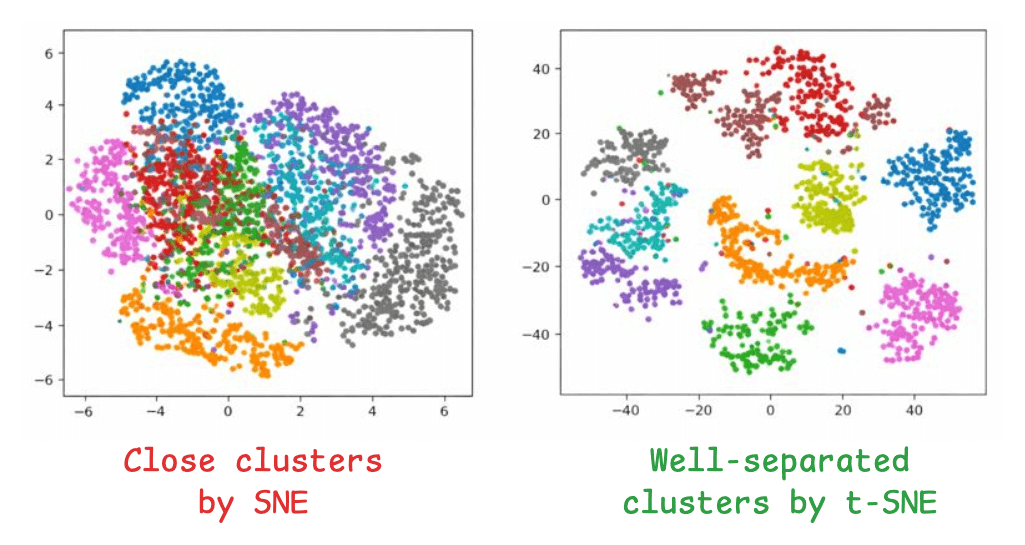
Clusters with SNE are close, without any defined segregation.
Clusters with t-SNE are well separated.
Today, let’s understand how exactly SNE differs from t-SNE.
A brief about tSNE
First, let’s briefly understand how SNE works.
The core objective is to project a given high-dimensional data into low-dimensions (mostly 2D) for visualisation.
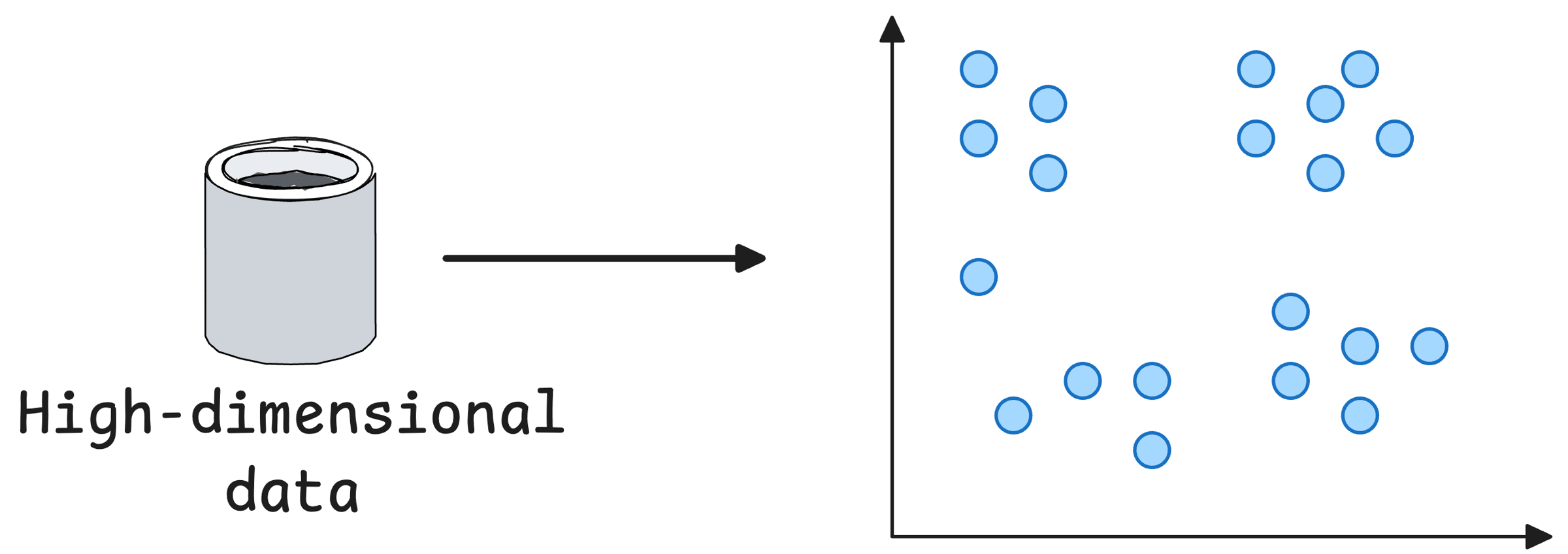
This is how we do it with the SNE algorithm:
Step 1) For every point (i) in the given high-dimensional data, plot Euclidean distances to all other points (j), which gives you a Gaussian-like probability distribution. For instance, consider the dark red point marked on the left below. Other red points that are closer to it have a higher probability of being i‘s neighbor than those that are far:
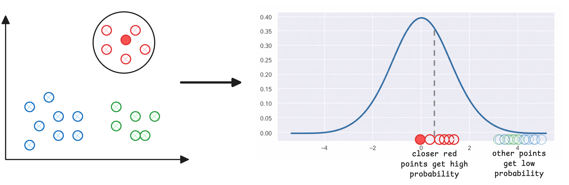
The above step assigns a neighbourhood distribution to every data point.
Step 2) Next, for every data point xᵢ in the given data (which is in high-dimensions), randomly initialize its counterpart yᵢ in 2D space. These will be our projections.
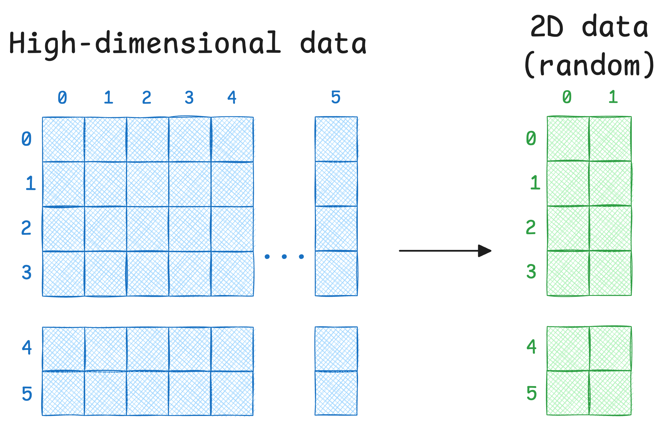
Step 3) Just like we created a distribution of Euclidean distances using high-dimensional data in Step 1, we create a Gaussian distribution of this random data.
Step 4) At this point, every data point (i) has a high-dimensional distribution and a random low-dimensional distribution. The objective is to match these two distributions so that the low-dimensional representation preserves the neighborhood structure of the high-dimensional data.
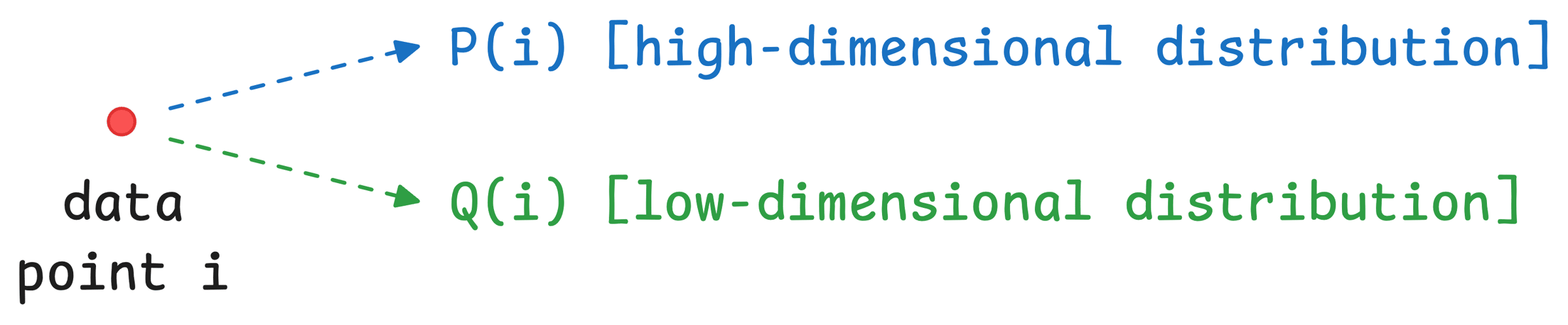
Using KL divergence as a loss function helps us achieve this. It measures how much information is lost when we use a distribution
Qto approximate distributionP.
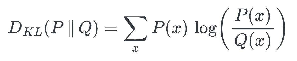
Ideally, we want to have the minimum loss value (which is zero), and this will be achieved when
P=Q.
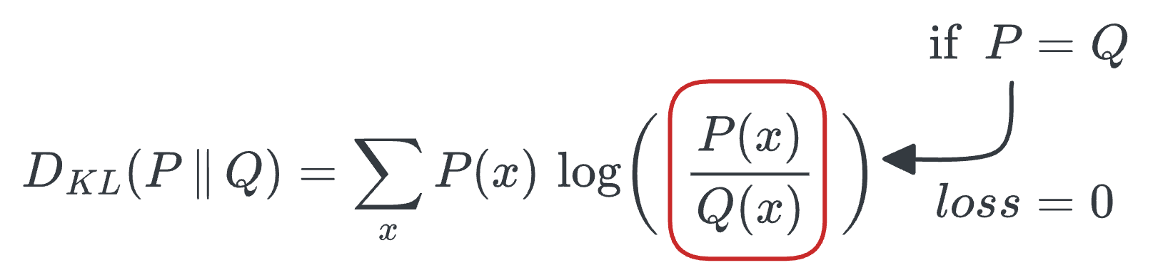
The model can be trained using gradient descent, and eventually, it generates projections that preserve the local neighborhood structure of the original high-dimensional data.
SNE results
The image below depicts a 2D visualization produced by the SNE algorithm on 256-dimensional handwritten digits:
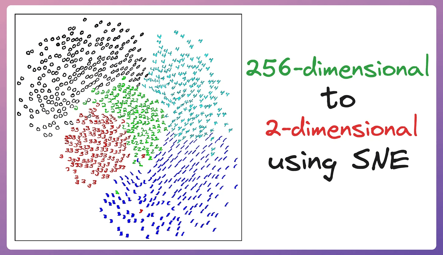
The projection looks good since properties like orientation, skew, and stroke thickness vary smoothly across the space within each cluster (clarified below):
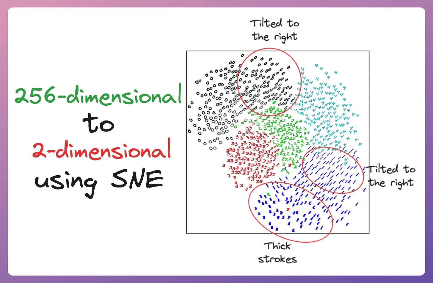
But the issue is that the clusters produced by SNE are not well separated.
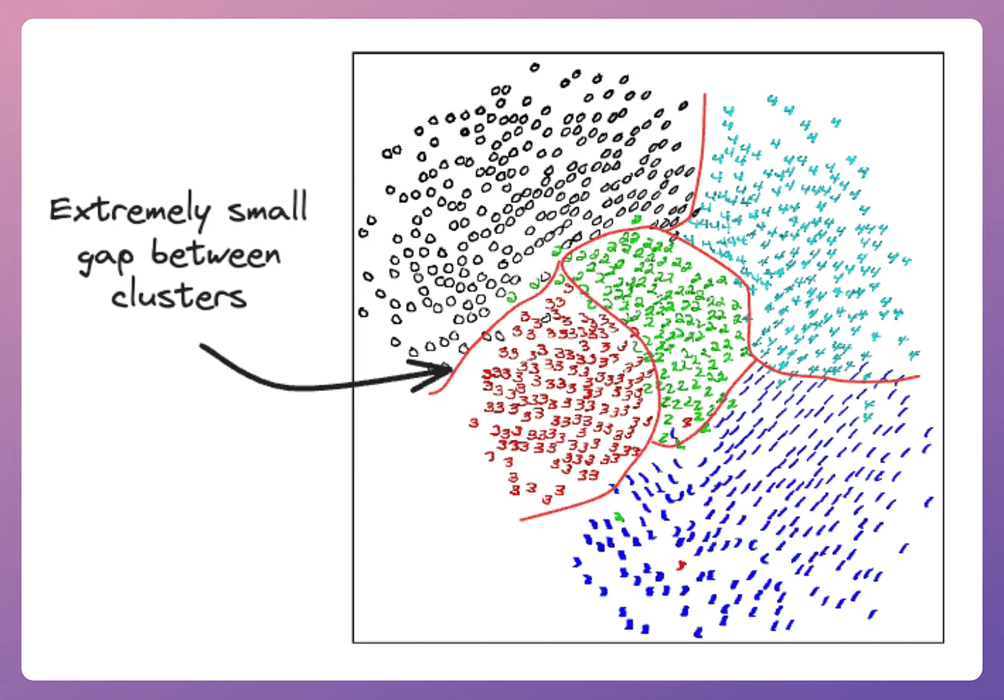
This is also called the crowding problem.
Solution implemented in t-SNE
To eliminate this issue, t-SNE was proposed, short for “t-distributed Stochastic Neighbor Embedding (t-SNE).”
Here’s the difference.
SNE uses a Gaussian distribution to define the low-dimensional probabilities. But we have already seen that it does not produce well-separated clusters.
The reason is that in high-dimensional space, there’s plenty of room for points to spread out. But when we squeeze everything into 2D, that room disappears.
Think of it like this: Imagine 100 people standing in a large hall (high-dimensional space). Now ask them to stand on a narrow sidewalk (2D space). Suddenly, everyone is cramped together.
The Gaussian distribution makes this worse because its tails drop off quickly. Distant points in high dimensions get mapped to very small probabilities, so the algorithm doesn’t push them far enough apart in 2D.
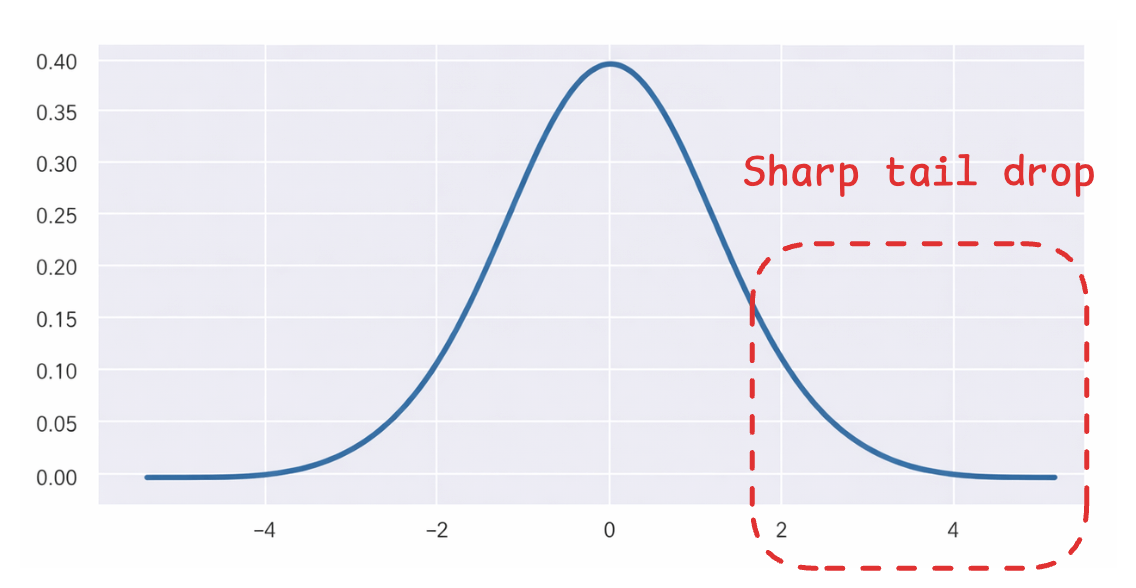
The solution to this is to use a distribution with heavier tails.
The Student t-distribution is a perfect fit for it (shown as the red distribution).

In simpler terms:
With a Gaussian, two points need to be close in 2D to have a moderate probability.
With a t-distribution, two points can be farther apart in 2D and still achieve the same probability
Notice the black horizontal line above to understand this (x-axis depicts distance).
This flexibility is crucial since the t-distribution allows moderate-distance points to spread out farther in 2D while still satisfying the probability constraints.
Close neighbors remain close, but everything else gets more room to spread out:
The following image depicts the difference this change brings:
As shown above:
SNE produces closely packed clusters.
t-SNE produces well-separated clusters.
And that’s why the t-distribution is used in t-SNE.
Beyond better cluster separation, the t-distribution offers computational advantages.
Evaluating the density of a point under a Student t-distribution is faster than under a Gaussian because we avoid computing expensive exponentials.
We went into much more detail in a beginner-friendly manner in the full article: Formulating and Implementing the t-SNE Algorithm From Scratch.
This article covers:
The limitations of PCA.
The entire end-to-end working of the SNE algorithm (an earlier version of t-SNE).
What does SNE try to optimize?
What are local and global structures?
Understanding the idea of
perplexityvisually.The limitations of the SNE algorithm.
How is t-SNE different from SNE?
Advanced optimization methods used in t-SNE.
Implementing the entire t-SNE algorithm by only using NumPy.
A practice Jupyter notebook for you to implement t-SNE yourself.
Understanding some potential gaps in t-SNE and how to possibly improve it.
PCA vs. t-SNE comparison.
Limitations of t-SNE.
Why is
perplexitythe most important hyperparameter of t-SNE?Important takeaways for using t-SNE.
Similar to this, we also formulated the PCA algorithm from scratch here: Formulating the PCA Algorithm From Scratch →
👉 Over to you: Can you identify a bottleneck in the t-SNE algorithm?
Thanks for reading!