

A good technical LLM interview question:
Your RAG chatbot is working as expected locally.
You deploy it behind a load balancer with 3 replicas.
Users report that it forgets what they just asked, and answers get worse with each restart.
Why did this happen?
(answer below)
A local setup has one process that owns everything.
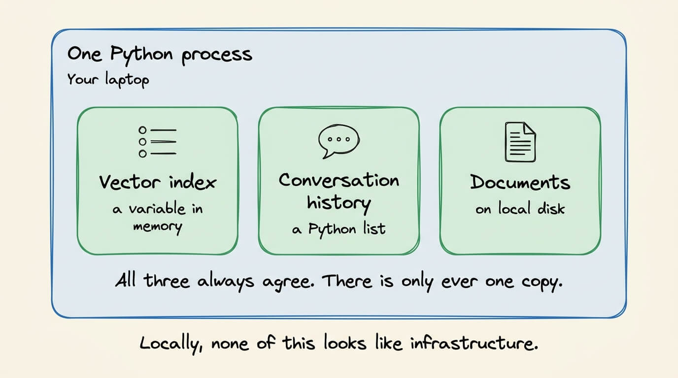
The vector index is a variable in memory.
Conversation history is a Python list.
The documents are on local disk.
You never treat any of them as infrastructure, because restarting rebuilds all three in seconds and there is only ever one copy.
The setup does not carry over to production directly.
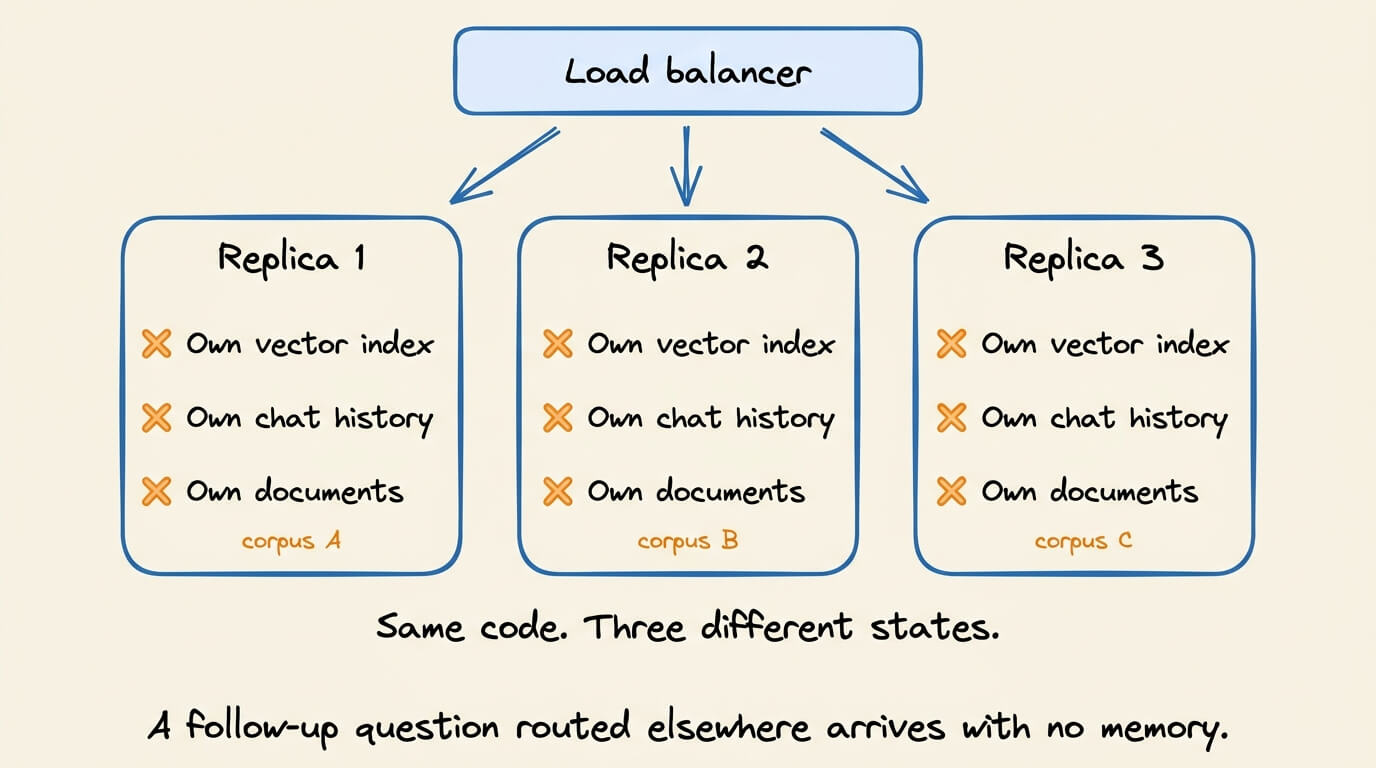
The vector index might disappear on restart, so the app re-embeds everything on boot and serves empty results until it finishes.
Conversation history may belong to one replica, so a follow-up routed elsewhere has no memory of the previous turn.
Documents could be on whichever container ingested them, so the three replicas hold three different corpora.
None of this is evident with one user and one process.
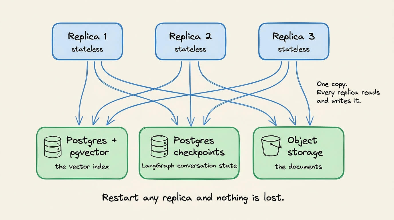
So the actual work in shipping RAG is not just the retrieval logic, but also storing the vector index, the conversation history, and the documents outside the app, where every replica reads and writes the same copy.
Which comes down to three requirements:
The vector store needs persistence and has to be reachable from every replica. pgvector inside Postgres keeps embeddings next to the rest of the data instead of adding another system to operate.
Conversation state has to be checkpointed outside the app. LangGraph writes its state to Postgres, so any replica can pick up a thread mid-conversation.
Docs need shared object storage, so ingestion happens once instead of once per replica.
If you get those three right, the retrieval logic you wrote in the notebook works unchanged.
To learn how all of it is wired together, Akamai’s GitHub has a working reference implementation.

rag-langgraph-k8s-quickstart is an airline policy Q&A assistant built with FastAPI, LangChain, and LangGraph. Terraform provisions the LKE cluster, a Postgres instance with pgvector for embeddings, a second Postgres for LangGraph checkpointing, and an object storage bucket for the policy documents, in one apply.
akamai-workshop-ai-inference covers the next step, running the model yourself instead of calling an API, with prefill and decode, KV cache tradeoffs, and continuous batching under real concurrency.
Both are available on Akamai’s new Developer Hub, alongside their tutorials and code samples.
It also links to Edge Case, their Discord, where four developer advocates architect and deploy a production app live every other Wednesday.
If you create a new Akamai Cloud account, you can also get $300 in credits for joining.
Join here: developers.akamai.com
Thanks to Akamai for partnering today!
Static vs. Dynamic vs. Continuous Batching in LLMs, clearly explained!
A modern GPU can run trillions of floating-point operations every second. Serving an LLM on one, you will often watch it run at a small fraction of that.
The reason is that generating a single token requires reading every weight in the model out of memory. That read dominates the time, and the compute units spend most of it waiting.
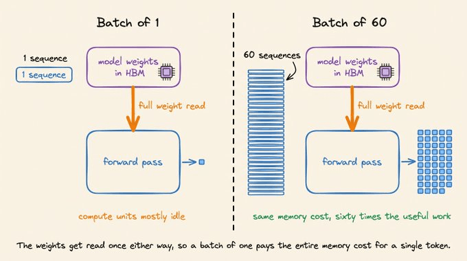
Batching is intended to solve that, wherein you load the weights once and push many sequences through the same pass so that the memory cost gets spread across all of them.
Every serving engine does this. What separates them is when the batch gets decided.
Static decides once, before the batch starts
Dynamic decides on a timer
Continuous decides again at every forward pass
That last one is where nearly all the throughput in modern serving comes from. The other two are worth understanding first, since each fails in a way the next is built to fix.
And today we are going to break down and understand each of them one by one.
Let’s begin!
Why batching exists
An A100 does roughly 312 teraFLOPs of BF16 math per second and moves about 2 terabytes per second out of memory. Decoding leans entirely on the second number.
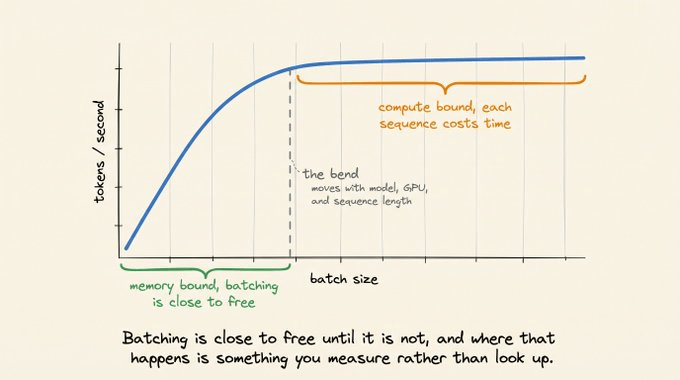
Reading the weights is the whole cost, and the compute sits idle waiting. That idle compute is free capacity, so a batch of sixty rides the same weight read as the batch of one did, and throughput climbs while the memory read time stays the same.
Note that, throughput climbs steeply with batch size, then flattens.
Below the bend you are memory bound, and batching is close to free
Above it you are compute bound, and each added sequence costs time
The bend moves with the model, the GPU, and the sequence length, so measure it on your own hardware.
Now, you might be thinking: if batching is this effective, why not batch as much as possible?
Well, with LLMs, that is harder than it sounds. Let’s understand why.
Why standard batching does not work in LLMs
Batching is older than LLMs. For a classifier or an embedding model, it is a packing problem.
Pad the inputs to a common length, stack them into one tensor, run one pass.
That works because three things hold. One pass produces the whole answer, no row depends on another, and every row’s cost is known before it starts.
This doesn’t work for autoregressive LLMs.
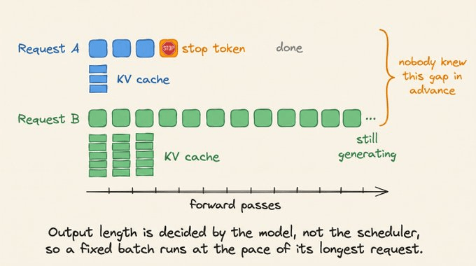
One pass produces one token, not the answer. A 400-token reply needs 400 forward passes.
Rows depend on their own history. Each pass writes into that request’s KV cache, which the next pass reads back.
Cost is unknown until it is over. The model decides by emitting a stop token, which can after 12 tokens or after 4,000.
Padding does not rescue this. It equalizes input width, not how long a request holds the GPU.
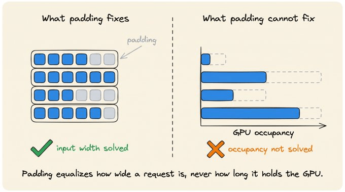
So a batch fixed at the start runs at the pace of its slowest member. The three strategies are three answers to that, in increasing order of how much they do about it.
Static batching
The simplest answer does nothing about it. Collect a fixed number of requests, run them together, and return everything when the last one finishes.
Here’s how the end state looks like:
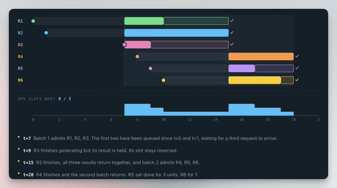
R3 stops generating at t=9 and sits on the GPU until t=15, because R2 is still running. That costs you twice:
Six units of latency for a user whose answer was already done
A held slot that a queued request could have used
Waste scales with higher output variance. Anyscale measured this on OPT-13B on a 40GB A100. Widening the spread of output lengths dropped static batching to roughly 81 tokens per second, while continuous batching held an order of magnitude higher.
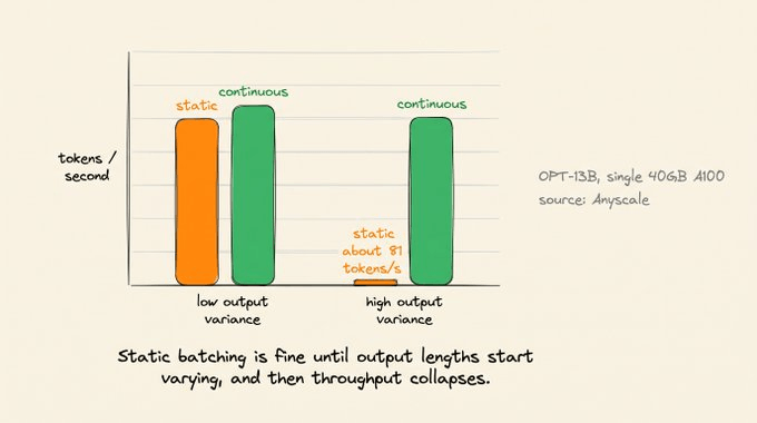
Still the right call sometimes. Static batching only looks bad when output lengths vary. Take that away and the slow-member problem goes with it.
Classification, embeddings, and scoring do exactly that. Each emits a fixed-size output, a label or a vector, so every request in the batch finishes at nearly the same step, and none waits on a straggler.
For that kind of work, static batching is simpler and gives up nothing.
Here’s how you configure static batching in vLLM:
from vllm import LLM, SamplingParams

llm = LLM(model="meta-llama/Llama-3.1-8B-Instruct")
outputs = llm.generate(prompts, SamplingParams(max_tokens=64))
llm.generate hands the engine the whole workload at once. Cap max_tokens, keep prompt sizes similar, and every sequence finishes at nearly the same step.
The Hugging Face pipeline API with a
batch_sizeargument is also static batching. Fine for evaluation scripts, poor for live traffic.
Dynamic batching
Static batching has a second cost. A request can wait a long time just to enter a batch.
If the batch size is 8 and only 5 have arrived, those 5 sit idle until three more show up.
Dynamic batching adds a timer. The batch fires on the size limit or when the window expires, whichever comes first.
Here’s how the end state looks like:
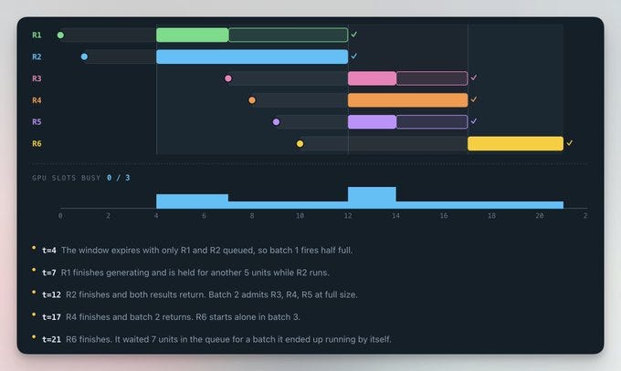
Batch 1 fires at t=4 (the fixed interval) with only R1 and R2, because the window expired before a third arrived. Both start four units earlier than static batching allowed.
It shortens the wrong wait. R1 finishes at t=7 and still waits until t=12, because R2 is not done.
Dynamic batching decides once per batch, then hands control to the engine until every member is done. For fixed-output models, that is a complete answer, which is why Triton ships it.
dynamic_batching {
  preferred_batch_size: [ 4, 8 ]
  max_queue_delay_microseconds: 100
}
preferred_batch_sizelists the sizes the scheduler tries to form.max_queue_delay_microsecondscaps how long a request waits for company.
Continuous batching
Both strategies so far treat a batch as one unit of work that starts and runs until every request in the batch has finished. That assumption is what still costs you, and continuous batching drops it.
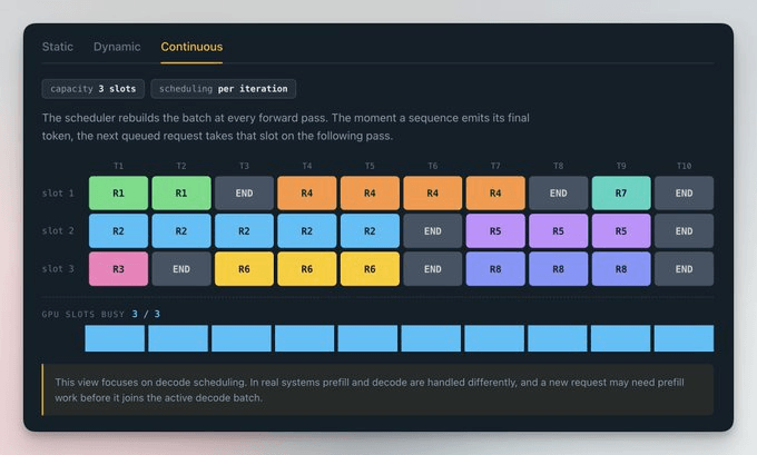
The scheduler runs one iteration, gets control back, and decides again. The moment a sequence emits its final token, it leaves the batch, and a waiting request takes that slot on the next pass.
The batch composition changes every iteration, which is why this is iteration-level scheduling. No slot waits for the slowest sequence, so the GPU stays saturated even when output lengths vary wildly.
This is how the end state looks like:
The limit is memory, not compute. Every active sequence holds a KV cache that grows with each token, and that cache, not the math, is what caps how many sequences fit.
On a 40GB A100 with a 13B model resident, only a handful of long sequences fit at once. When the pool runs out, the scheduler evicts a running request and recomputes it later.
That looks like the GPU running out of headroom, when it is really the same prefill computed twice.
👉 Every engine ships continuous batching under a different name: vLLM, SGLang, and TGI call it that, TensorRT-LLM calls it in-flight batching, LMDeploy calls it persistent batching.
Chunked prefill
Rebuilding the batch every pass fixes the slow-member problem and introduces a new one, which users see as a stutter.
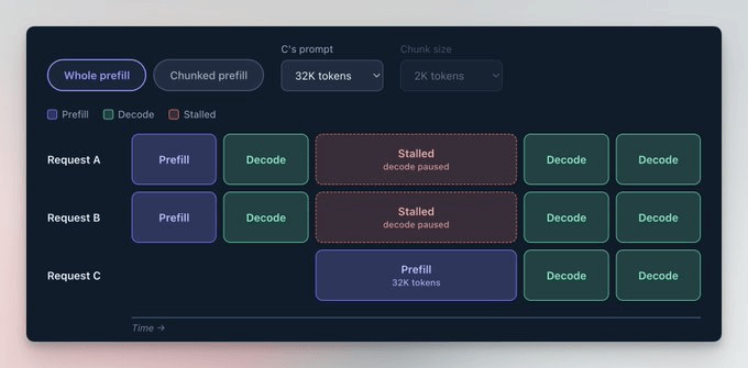
A joining request is prefilled in one iteration. A 32K-token prompt is one large, compute-heavy pass that every active decode waits behind, so output pauses mid-sentence because someone else pasted a long document.
Here’s how things look without and with chunked prefill.
Whole prefill:
Chunked prefill:
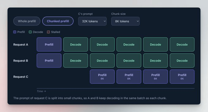
(prompt of request C is broken down into smaller chunks of 2k tokens each)
Split the prompt across iterations. Chunked prefill breaks the prompt into fixed-size token ranges scheduled over several passes, each extending the request’s KV cache.
The attention math is unchanged, since later chunks attend to what earlier chunks processed. The first token arrives after the final chunk.
Prefill is compute-bound, and decode is memory-bound, so one batch containing both uses both parts of the chip.
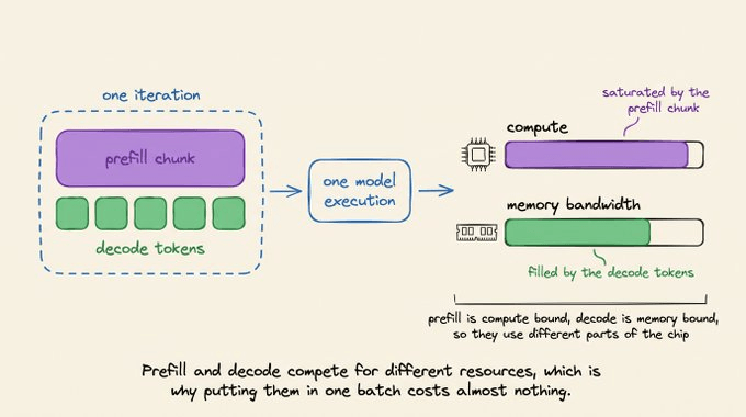
When choosing values, note that:
Smaller chunks give the scheduler more opportunities to run decodes, reducing ITL spikes for active requests.
Larger chunks process the new prompt more efficiently and usually improve the TTFT, but active decodes may wait longer between tokens.
Chunks that are too small can lower GPU utilization and add attention overhead because later chunks must reread KV cache entries created by earlier chunks.
Chunked prefill is on by default in vLLM V1, where --max-num-batched-tokens caps tokens per iteration. SGLang uses --chunked-prefill-size, and -1 disables it.
vLLM:
vllm serve meta-llama/Llama-3.1-8B-Instruct \
  --max-num-batched-tokens 8192
SGLang:
sglang serve --model-path meta-llama/Llama-3.1-8B-Instruct \
  --chunked-prefill-size 8192
👉 There is no universal best chunk size. It depends on the model, the GPU, your prompt length distribution, and which latency metric your SLO measures.
Conclusion
The three strategies differ only in when they fix the batch, and each answers a different workload shape.
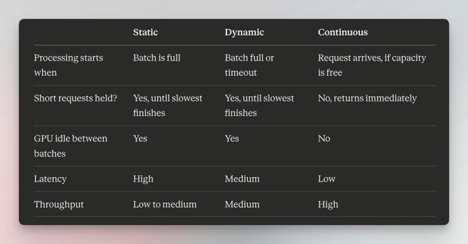
For live traffic with variable output lengths, continuous batching is the only one that holds up, and every major engine gives it to you by default.
This whole article rests on one fact about GPUs: a forward pass is bottlenecked on reading weights out of memory, not on the math.
We have written a detailed article on how a GPU works →
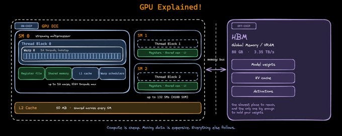
It builds up from first principles why memory and compute compete, why that gap exists in the hardware, and what makes a workload memory-bound in the first place. It needs no prior background, and it is the natural prequel to everything above.
Stay tuned for more.
Good day!