
Testing, Security and Sandboxing in MCP Workflows (With Implementation)
The full MCP blueprint.

In today’s newsletter:
Testing, Security, and Sandboxing in MCP Workflows.
Opik Bounty Program: Get paid to contribute to open-source.
Two techniques to extend the context length of LLMs.
Testing, Security and Sandboxing in MCP Workflows
Part 6 and Part 7 of the MCP crash course are now available, where we explain testing, security and sandboxing in MCP Workflows.
More specifically, they cover:
What is testing in MCP, and how does the MCP Inspector help?
Significance of security in MCP systems
The key vulnerabilities in MCP
Real-world threats like prompt injection, tool poisoning, server impersonation, and excessive capability exposure.
How to define and enforce boundaries using MCP roots.
Possible solutions to address the key threats
What is sandboxing and why is it critical?
Fully containerizing a FastMCP server using Docker
How to enforce runtime limits and security boundaries with Docker flags?
How to connect Claude Desktop, Cursor, and custom clients to sandboxed containers?
Each topic will be backed by examples and walkthroughs so you not only understand the theory, but can also implement it confidently in your own stack.
Just like our past series on RAG and AI Agents, this series is both foundational and implementation-heavy, walking you through everything step-by-step.
Here’s what we have done so far:
In Part 1, we introduced:
Why context management matters in LLMs.
The limitations of prompting, chaining, and function calling.
The M×N problem in tool integrations..
And how MCP solves it through a structured Host–Client–Server model.
In Part 2, we went hands-on and covered:
The core capabilities in MCP (Tools, Resources, Prompts).
How JSON-RPC powers communication.
Transport mechanisms (Stdio, HTTP + SSE).
A complete, working MCP server with Claude and Cursor.
Comparison between function calling and MCPs.
In Part 3, we built a fully custom MCP client from scratch:
How to build a custom MCP client and not rely on prebuilt solutions like Cursor or Claude.
What the full MCP lifecycle looks like in action.
The true nature of MCP as a client-server architecture, as revealed through practical integration.
How MCP differs from traditional API and function calling, illustrated through hands-on implementations.
In Part 4, we built a full-fledged MCP workflow using tools, resources, and prompts.
What exactly are resources and prompts in MCP?
Implementing resources and prompts server-side.
How tools, resources, and prompts differ from each other.
Using resources and prompts inside the Claude Desktop.
A full-fledged real-world use case powered by coordination across tools, prompts, and resources.
In Part 5, we integrated Sampling into MCP workflows.
What is sampling, and why is it useful?
Sampling support in FastMCP
How does it work on the server side?
How to write a sampling handler on the client side?
Model preferences
Use cases for sampling
Error handling and some best practices
MCP is already powering real-world agentic systems.
And in this crash course, you’ll learn exactly how to implement and extend it, from first principles to production use.
Read the first two parts here:
Opik Bounty Program: Get paid to contribute to open-source

Comet's bounty program rewards developers for contributing to Opik, their open-source AI evaluation and observability platform.
Whether you're building your portfolio, exploring new tech, or aiming to contribute to top open-source projects, this is a great opportunity.
Thanks to Comet for opening these opportunities and partnering today!
Two techniques to extend the context length of LLMs
Consider this:
GPT-3.5-turbo had a context window of 4,096 tokens.
Later, GPT-4 took that to 8,192 tokens.
Claude 2 reached 100,000 tokens.
Llama 3.1 → 128,000 tokens.
Gemini → 1M+ tokens.
We have been making great progress in extending the context window of LLMs.
Today, let's understand some techniques that help us unlock this.
What's the challenge?
In a traditional transformer, a model processing 4,096 tokens requires 64 times more computation (quadratic growth) than one handling 512 tokens due to the attention mechanism.

Thus, having a longer context window isn't just as easy as increasing the size of the matrices, if you will.
But at least we have narrowed down the bottleneck.
If we can optimize this quadratic complexity, we have optimized the network.
A quick note: This bottleneck was already known way back in 2017 when transformers were introduced. Since GPT-3, most LLMs have utilized non-quadratic approaches for attention computation.
1) Approximate attention using Sparse Attention
Instead of computing attention scores between all pairs of tokens, sparse attention limits that to a subset of tokens, which will reduce the computations.
There are two common ways:
Use local attention, where tokens attend only to their neighbors.
Let the model learn which tokens to focus on.

As you may have guessed, there's a trade-off between computational complexity and performance.
2) Flash Attention
This is a fast and memory-efficient method that retains the exactness of traditional attention mechanisms.

The whole idea revolves around optimizing the data movement within GPU memory. Here are some background details and how it works.
In a GPU:
A thread is the smallest unit of execution.
A group of threads is called a block.
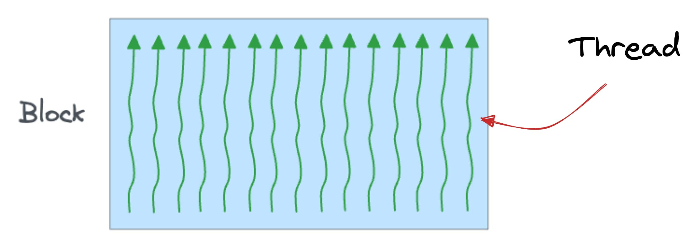
Also:
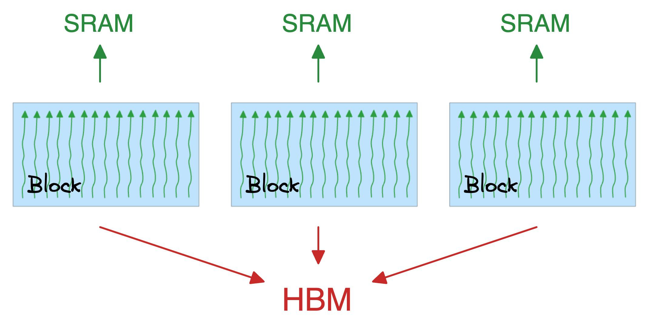
A block executes the same kernel (function, to simplify) and its threads cooperate by sharing a fast memory block called SRAM.
Also, all blocks together can access a shared global memory block in the GPU called HBM.
A note about SRAM and HBM:
SRAM is scarce but extremely fast.
HBM is much more abundant but slow (typically 8-15x slower).
The quadratic attention and typical optimizations involve plenty of movement of large matrices between SRAM and HBM:
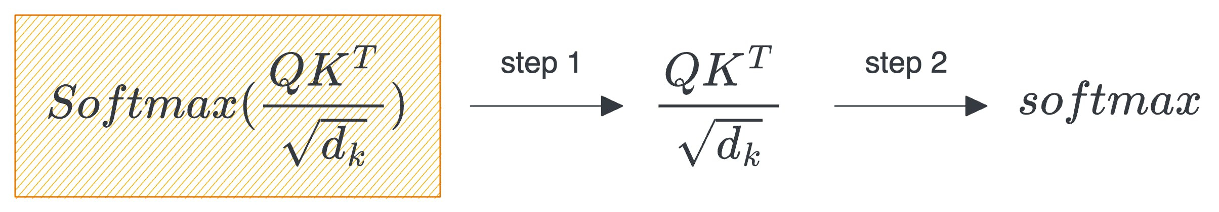
First, the product of query (Q) and key (K) is distributed to threads, computed, and brought back to HBM.
Next, the above result is again distributed to threads to compute the softmax of the product and brought back to HBM once it is done.
Flash attention reduces repeated movements by utilizing SRAM to cache the intermediate results.
This way, redundant movements are reduced, and typically, this offers a speedup of up to 7.6x over standard attention methods.
Also, it scales linearly with sequence length, which is also great.
While reducing the computational complexity is crucial, this is not sufficient.
See, using the above optimization, we have made it practically feasible to pass longer contexts without drastically increasing the computation cost.
However, the model must know how to comprehend longer contexts and the relative position of tokens.
That is why selecting the right positional embeddings is crucial.

Rotary positional embeddings (RoPE) usually work the best since they preserve both the relative position and the relation.
If you want to learn more about RoPE, let us know. We can cover it in another issue.
In the meantime, if you want to get into the internals of CUDA GPU programming and understand the internals of GPU, how it works, and learn how CUDA programs are built, we covered it here: Implementing (Massively) Parallelized CUDA Programs From Scratch Using CUDA Programming.
Thanks for reading!