

Fine-tune any LLM directly from Claude!
We built a Hugging Face fine-tuning studio that lets you fine-tune any LLM directly from Claude:
The app connects to the HF Hub for model and dataset search. It handles chat template formatting for the training data, and lets you configure LoRA rank, quantization, batch size, and learning rate directly from Claude.
Training runs on HF’s GPU infra via AutoTrain.
Once training finishes, you can also chat with your fine-tuned model (or any other LLM on HF) directly from Claude.
The studio’s built with the mcp-use SDK, an open-source full-stack framework to build MCP Apps for Agents.
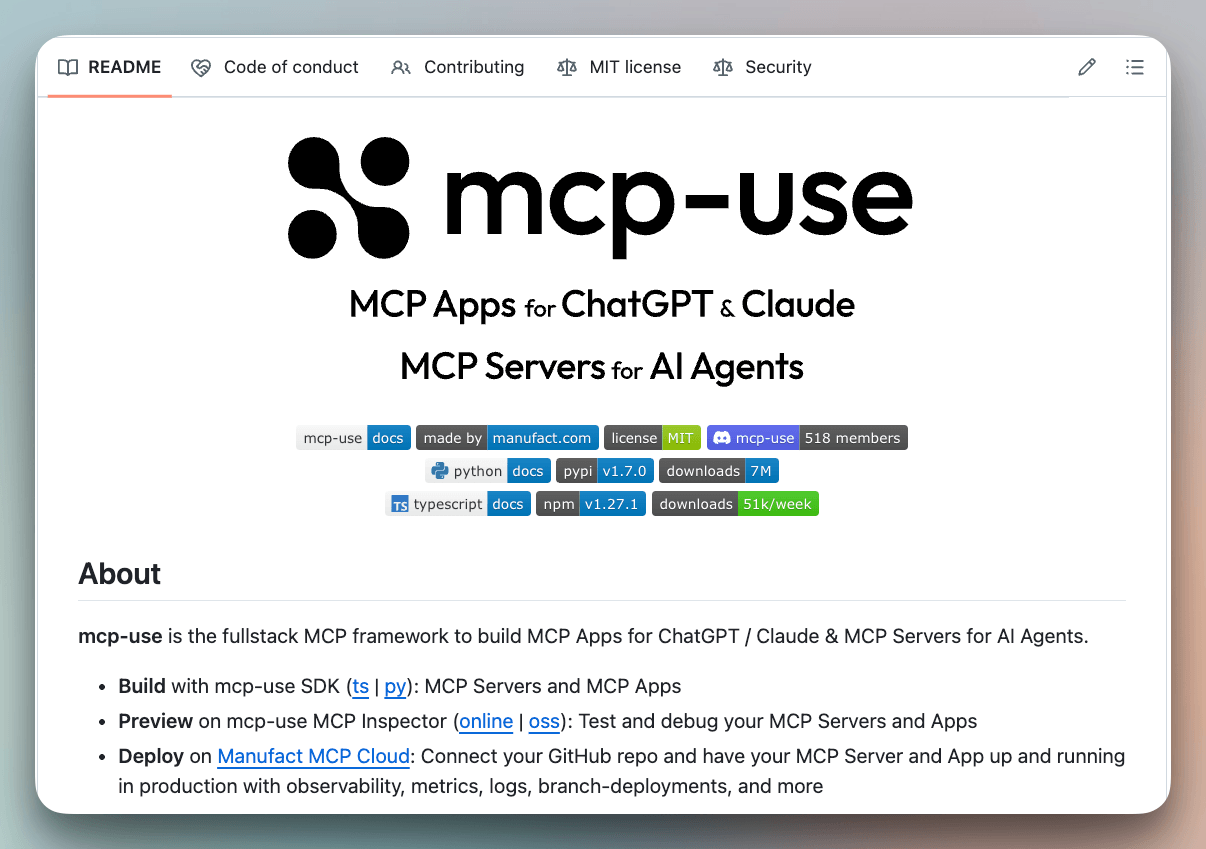
In mcp-use, any MCP tool can be associated with a UI.
You define a tool handler, create a React component, and the mcp-use framework handles the tool registration, prop mapping between server and widget, bundling, and hot reload during development.
The widgets follow the MCP Apps standard, inspired by OpenAI’s Apps SDK.
You can find the mcp-use GitHub repo here →
And you can find the code for this fine-tuning studio here →
The four types of agent loops
Loop engineering keeps getting talked about as one thing, when it’s actually a choice between four structures, each fitting a different kind of task.
It means designing the system that steers the agent, instead of steering it by hand, move by move.
That system always answers two questions: what starts a run, and what decides the work is done.
In a hand-run session, the human answers both, every single time. Each loop type moves more of that into the system.
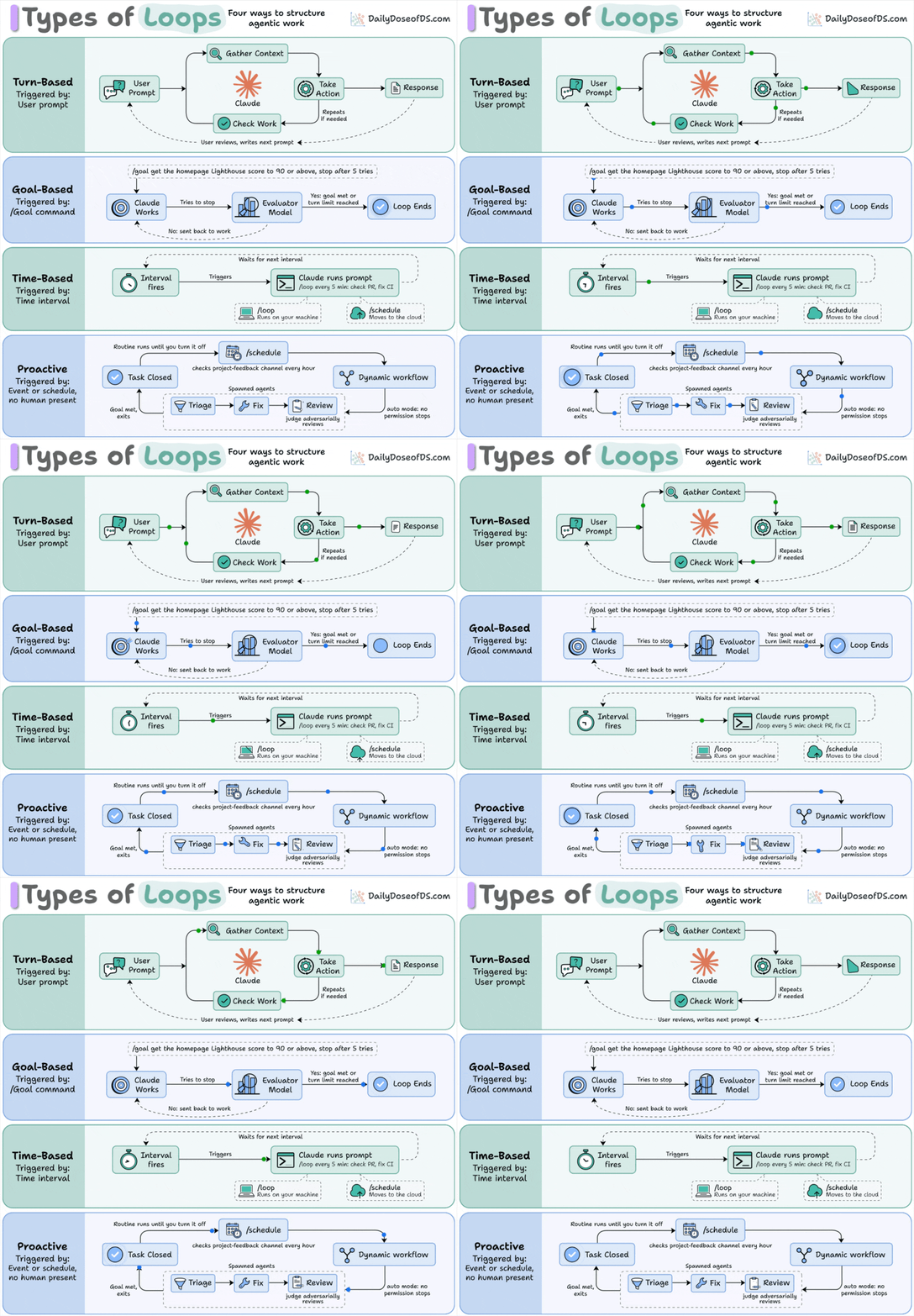
Here’s each type, what triggers it, and when to reach for it.
#1) Turn-based loops, triggered by a user prompt.
The agent gathers context, acts, and checks its work inside a single turn. Then a human reviews the output and writes the next prompt.
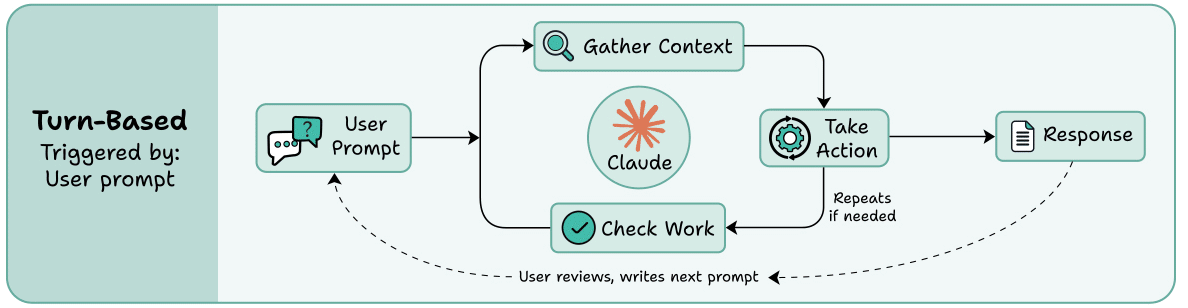
Use this when requirements are still forming and every output changes what the next prompt should ask for.
#2) Goal-based loops, triggered by a /goal command that carries success criteria and a budget, like “get the homepage Lighthouse score to 90, stop after 5 tries.”
When the agent tries to stop, an evaluator model checks whether the goal is met, and it sends it back to work.

Use this when the outcome is measurable but the path there doesn’t need human attention.
#3) Time-based loops, triggered by a clock.
An interval fires, the agent runs a fixed prompt like “check the PR, fix CI,” then waits for the next tick. The /loop command runs on the local machine, and /schedule moves it to the cloud so it survives a closed laptop.

Use this for recurring work where the task is known in advance and only the timing repeats.
#4) Proactive loops, triggered by an event or schedule with no human present.
A routine watches a channel and spawns a workflow when something needs handling. That workflow runs a triage agent, a fix agent, and a reviewer who adversarially judges the work before the task closes.

Use this for standing responsibilities where nobody can predict what will come in, only that something will.
Each type hands off one more job than the last. Turn-based keeps both jobs with the human, goal-based automates the checking, time-based automates the trigger, and proactive automates both while deciding the workflow shape at runtime.
So the mapping question isn’t which loop is most advanced. It’s whether the task is exploratory, measurable, recurring, or standing.
The more you hand off, the less you monitor yourself.
We wrote a full breakdown on loop engineering.
NVIDIA researchers built a new transformer variant
One small change to the layers made:
decoding 1.7x faster
long-reasoning accuracy up 6.5 points
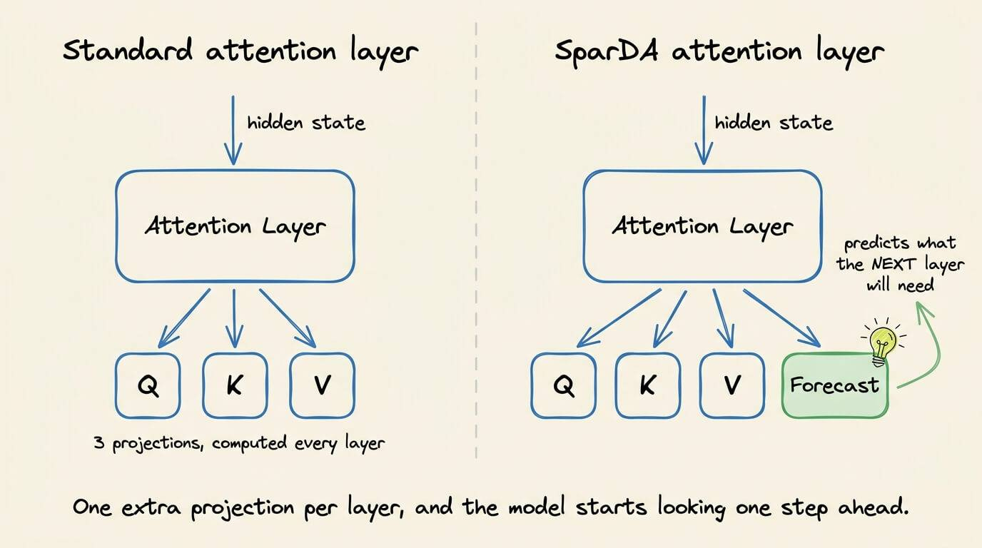
In a typical transformer architecture, every attention layer computes Q, K, and V.
NVIDIA’s tweak adds a fourth projection, which predicts what the next layer will need.
To understand why they did this, let’s first see what happens in a Transformer architecture during inference right now.
Sparse attention was an attempt to handle long-context inference. Instead of attending to every cached token, modern designs score the KV cache in blocks, keep the top-k, and attend only to those.
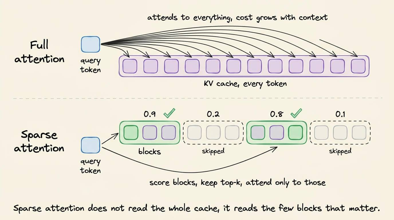
That cuts attention compute and bandwidth, but this still leaves us with two problems.
> First, the KV cache still grows with every generated token.
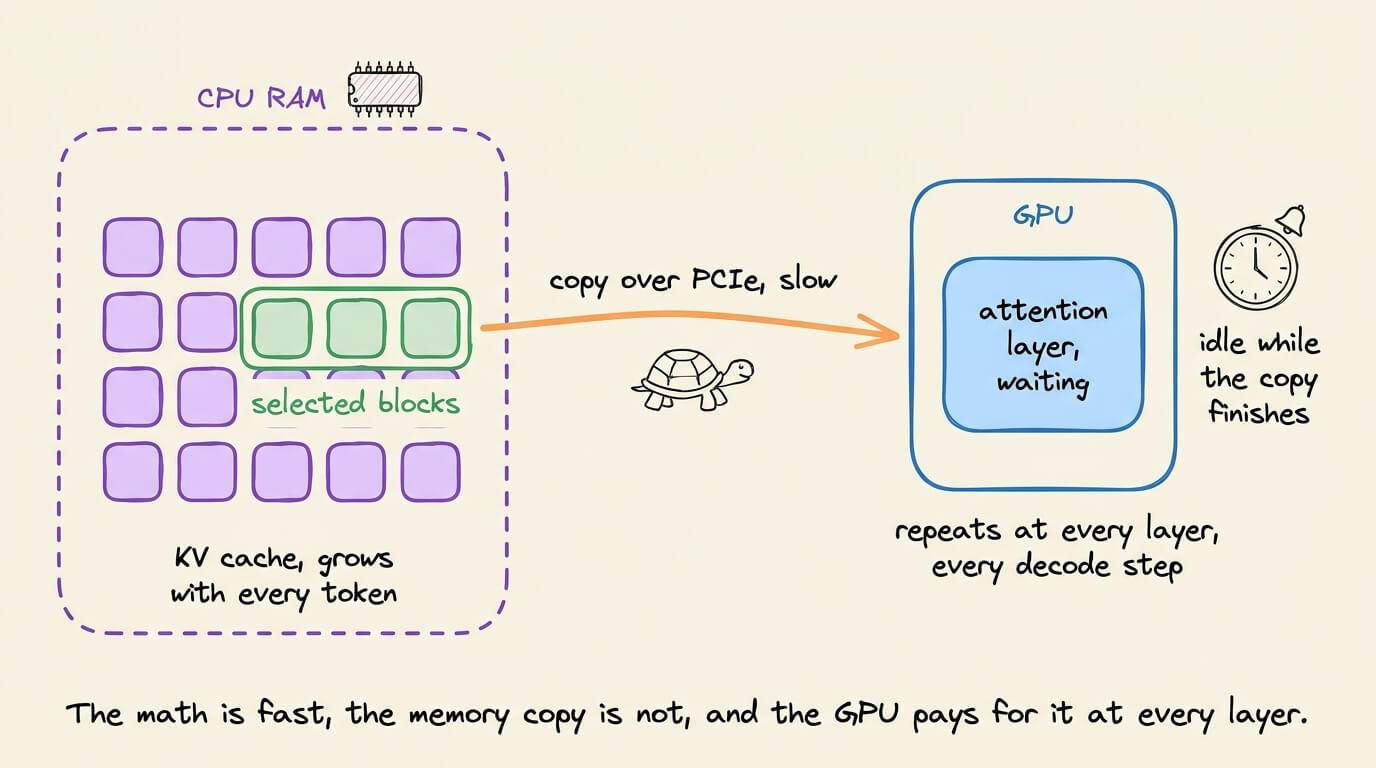
At 100K+ context, it no longer fits in GPU memory and gets offloaded to CPU RAM.
Now every layer must first copy its selected KV blocks from CPU memory back to the GPU. That copy is slow, the GPU sits idle while it waits, and the stall repeats at every layer of every decode step.
> Second, the selection step itself is not free.
Standard selectors score every candidate block with every query head in a GQA group (grouped-query attention, where several query heads share one KV head), then softmax each head’s scores and sum them across the group.
During decode, the sparse attention itself is cheap because there is only one query token.
But the expensive part is deciding which blocks to attend to, and that cost keeps growing with context length.
Both problems trace back to the same design in today’s sparse attention methods, i.e., the attention query drives the block selection.
Selection needs the query vector Q, and Q only exists once its layer is already running. By then, it’s too late to fetch anything early.
The query also drags its multi-head layout into selection, so all that scoring computation runs just to make one top-k decision.
A recent paper from NVIDIA and MIT called SparDA breaks this coupling with one architectural change.
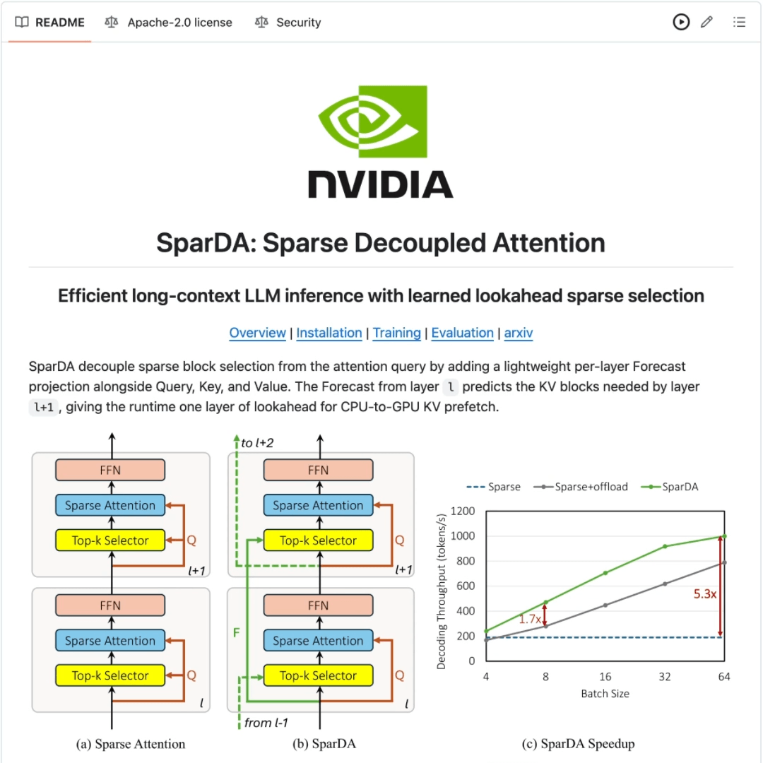
Each layer now emits four projections instead of three:
↳ Q, K, V, and a Forecast.
The Forecast from layer L predicts which KV blocks layer L+1 will need.
Layer L+1’s own query performs the sparse attention over those selected blocks.
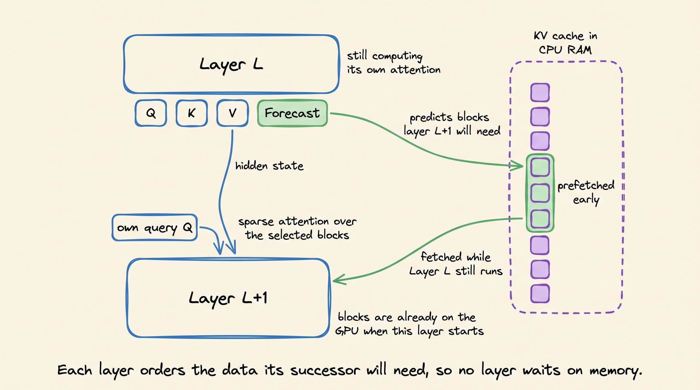
This one change fixes both problems.
Since the next layer’s block set is known while the current layer is still computing, the runtime fetches those blocks from CPU memory on a separate CUDA stream.
The copy overlaps with the current layer’s compute, so the GPU no longer waits for it.
And since the Forecast is separate from the attention query, it doesn’t need one score per query head.
SparDA uses one Forecast head per GQA group, which removes the per-query-head scoring loop and skips the softmax step entirely.
DeepSeek did something similar in DSA, where a small indexer picks important tokens instead of the query doing it.
SparDA applies the same idea to blocks and adds the prefetch angle that DSA doesn’t touch.
The cost of the change is small.
The Forecast adds just 33.5M parameters on an 8B model (0.41%), and only those projections are trained, using a KL loss that matches the original selector’s block distribution.

On MiniCPM4.1-8B and NOSA-8B, accuracy matches or beats the sparse baseline, with NOSA-8B gaining +6.5 on long reasoning.
Prefill runs up to 1.25x faster and decode up to 1.7x faster than the sparse offload baseline.
There’s one more benefit.
Because prefetch hides the offload cost, most of the KV cache can live in CPU RAM, and the freed GPU memory fits much bigger batches, pushing decode throughput up to 5.3x over the non-offload sparse baseline.
That said, this lookahead will only pay off during decode with CPU offload. During prefill, all keys already live on the GPU, so the gain there comes purely from the cheaper selection.
Here’s the paper: https://arxiv.org/abs/2606.04511
We wrote a first-principles breakdown of how the KV cache works. It walks through why the model stores keys and values at all, why the cache grows with every token, and a comparison of LLM generation speed with and without KV caching.
Good day!