The Most Common Way a Continuous Probability Distribution is Misinterpreted

The difference between probability density function and probability.

Dec 13, 2023

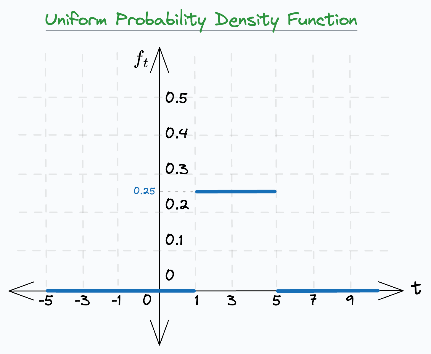
Consider the following probability density function of a continuous probability distribution. Say it represents the time one may take to travel from point A to B.

For simplicity, we are assuming a uniform distribution in the interval [1,5].
Essentially, it says that it will take somewhere between 1 and 5 minutes to go from A to B. Never more, never less.

Thus, the probability density function (PDF) can be written as follows:

Answer the following question for me:

Q) What is the probability that one will take precisely three minutes P(T=3) to reach point B?

A) 1/4 (or 0.25)
B) Area under the curve from t=[1,3].
C) Area under the curve from t=[3,5].

Decide on an answer before you read further.

To be honest, all of the above answers are wrong.

The correct answer is ZERO.

And I intentionally kept only wrong answers here so that you never forget something fundamentally important about continuous probability distributions.

Let’s dive in!

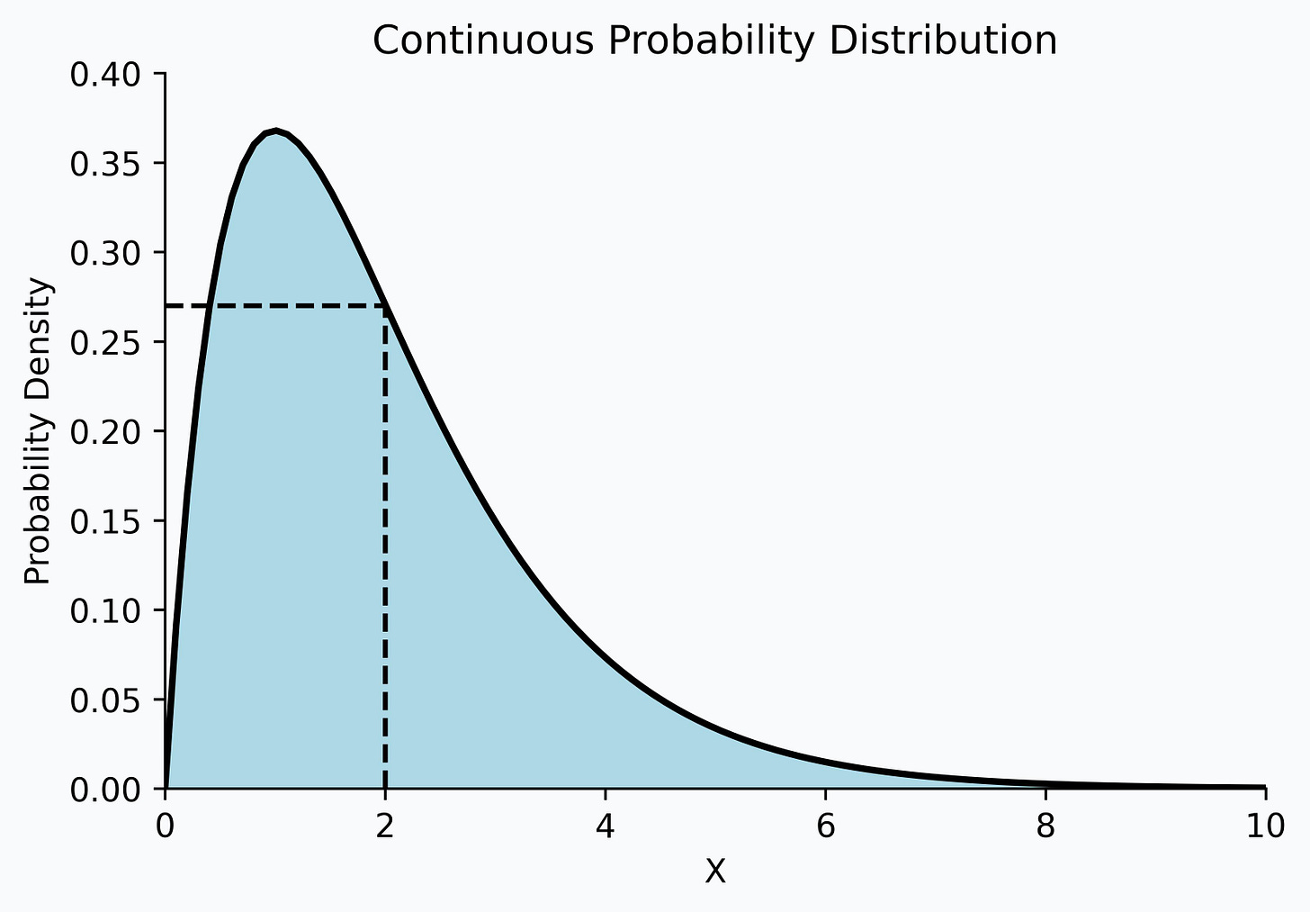
The probability density function of a continuous probability distribution may look as follows:

Some conditions for this probability density function are:

It should be defined for all real numbers (can be zero for some values).

This is in contrast to a discrete probability distribution which is only defined for a list of values.

The area should be 1.

The function should be non-negative for all real values.

Here, many folks often misinterpret that the probability density function represents the probability of obtaining a specific value.

For instance, by looking at the above probability density function, many incorrectly conclude that the probability of the random variable X being 2 is close to 0.27.

But contrary to this common belief, a probability density function:

DOES NOT depict the probabilities of a specific value.
is not meant to depict a discrete random variable.

Instead, a probability density function:

depicts the rate at which probabilities accumulate around each point.
is only meant to depict a continuous random variable.

Now, there are infinitely possible values that a continuous random variable may take.

So the probability of obtaining a specific value is always zero (or infinitesimally small).

Thus, answering our original question, the probability that one will take three minutes to reach point B is ZERO.

So what is the purpose of using a probability density function?

In statistics, a PDF is used to calculate the probability over an interval of values.

Thus, we can use it to answer questions such as…

What is the probability that it will take between:
- 3 to 4 minutes to reach point B from point A, or,
- 2 to 4 minutes to reach point B from point A, and so on…

And we do this using integrals.

More formally, the probability that a random variable X will take values in the interval [a,b] is:

Simply put, it’s the area under the curve from [a,b].

From the above probability estimation over an interval, we can also verify that the probability of obtaining a specific value is indeed zero.

By substituting b=a, we get:

To summarize, always remember that in a continuous probability distribution:

The probability density function does not depict the exact probability of obtaining a specific value.
Estimating the probability for a precise value of the random value makes no sense because it is infinitesimally small.
Instead, we use the probability density function to calculate the probability over an interval of values.

Any further follow-up questions? Feel free to reach out :)

👉 If you liked this post, don’t forget to leave a like ❤️. It helps more people discover this newsletter on Substack and tells me that you appreciate reading these daily insights.