

In today’s newsletter:
The next AI inference architecture, clearly explained (4x faster than GPUs).
Autoregressive LLMs vs. diffusion LLMs, clearly explained.
The next AI inference architecture, clearly explained (4x faster than GPUs)
Everything you need to understand why LLM decode waits on memory, and how a dataflow chip removes that wait. It covers the memory-bandwidth ceiling, kernel boundaries, the limits of kernel fusion, spatial mapping, memory tiers, disaggregated prefill and decode, and a hands-on speed test of GLM-5.3, a Mixture-of-Experts model on SambaNova Cloud.
A GPU runs an LLM as a long chain of small programs called kernels.
Even for a small Llama model, that chain has about a hundred kernels for every token the model generates.
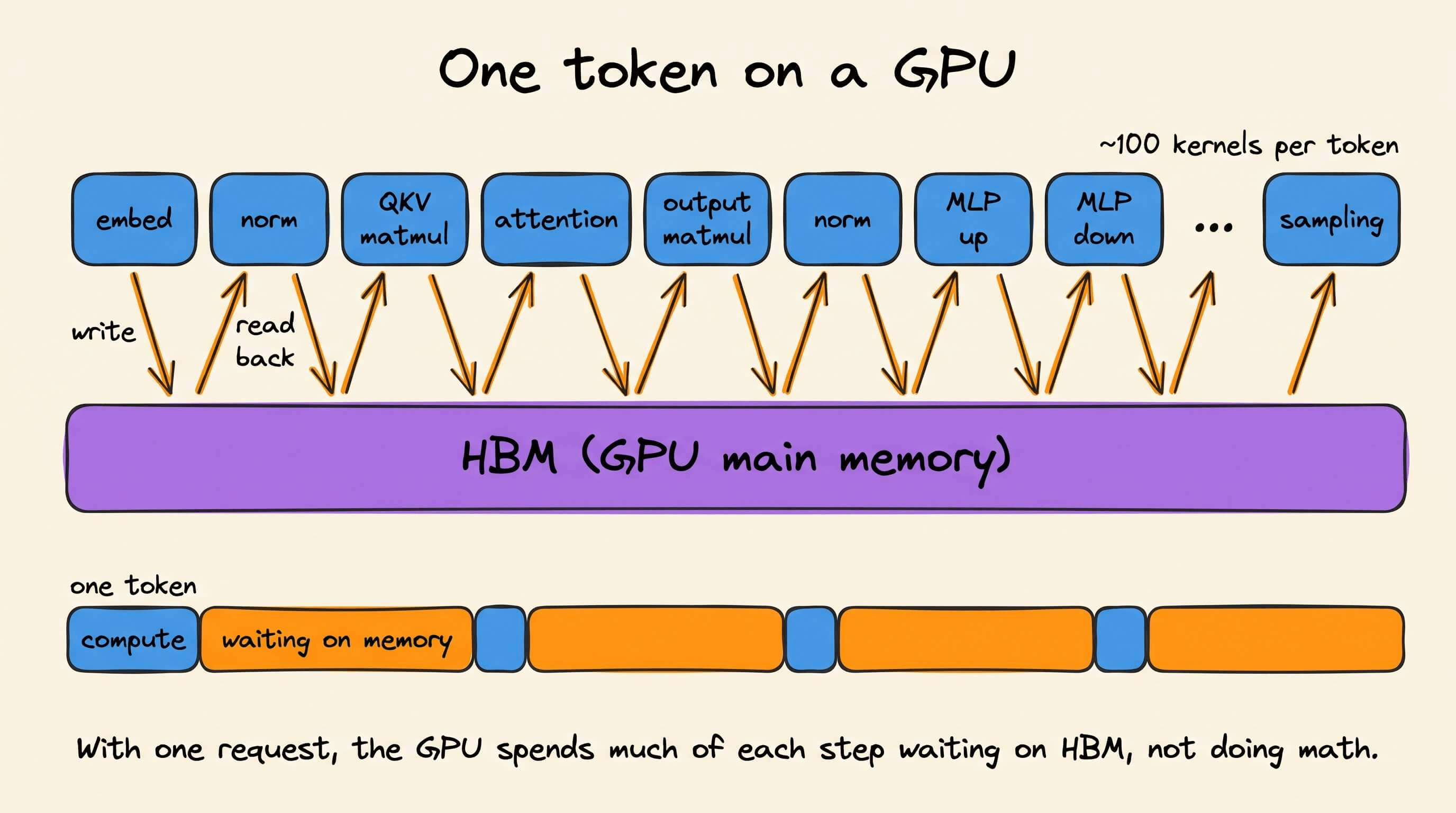
Each kernel writes its result to HBM, the GPU’s main memory, and the next kernel reads it back. With one request at a time, the chip spends much of each step waiting on memory instead of doing math.
AI agents suffer the most due to this. Anthropic reports that its agents use about 4x the tokens of a chat, and multi-agent systems use about 15x.
A dataflow chip, like SambaNova’s RDU, is a processor designed to pass each result straight to the next step on the chip, which minimizes trips to main memory. On 16 of SambaNova’s SN40L chips, this approach runs Llama 3.1 8B at about 1,100 tokens/s.
The visual below shows how this differs from a GPU:
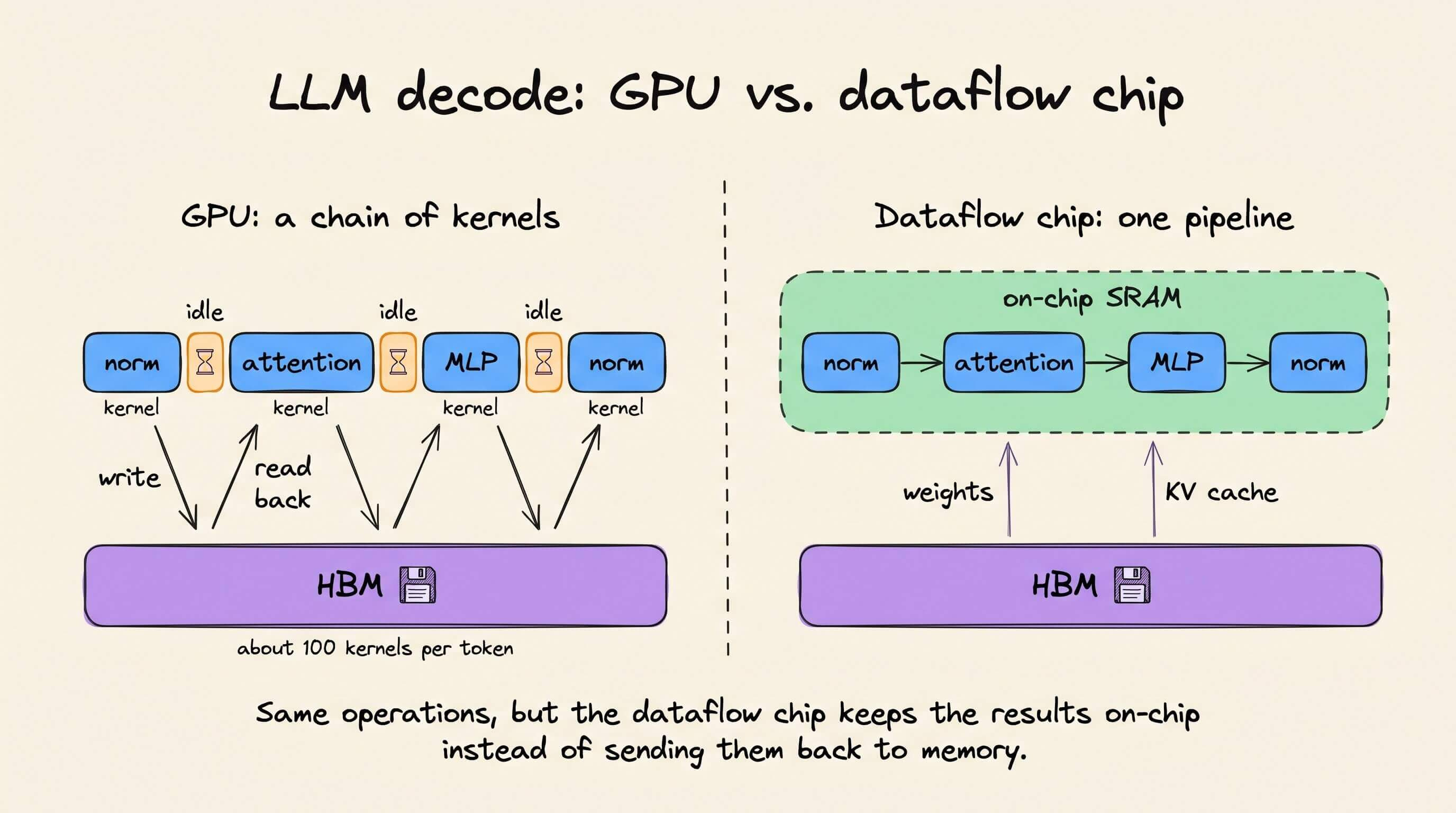
So today, let’s understand why a GPU leaves much of its memory bandwidth unused during decode, why kernel fusion only goes so far, and how SambaNova’s RDU runs a whole decoder layer as one pipeline that keeps results in on-chip SRAM.
We’ll end with a hands-on speed test of GLM-5.3, a Mixture-of-Experts model now running on SambaNova Cloud.
Prefill vs. decode in agent workloads
An agent works in a loop. It asks the model for the next action, runs a tool, adds the result to its context and repeats.
Every model call has two phases.
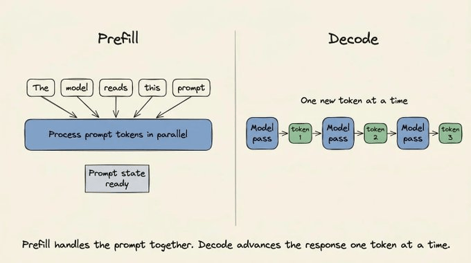
Prefill reads the whole prompt in parallel and builds the KV cache,
And decode then writes the answer one token at a time.
A recent study traced this loop on benchmarks like SWE-bench Pro and Terminal-Bench. Model inference took 71% to 98% of the total runtime.
Each turn reuses almost all of the last turn’s context, so prefix caching skips most of the prefill work.
Memory-bandwidth ceiling for decode
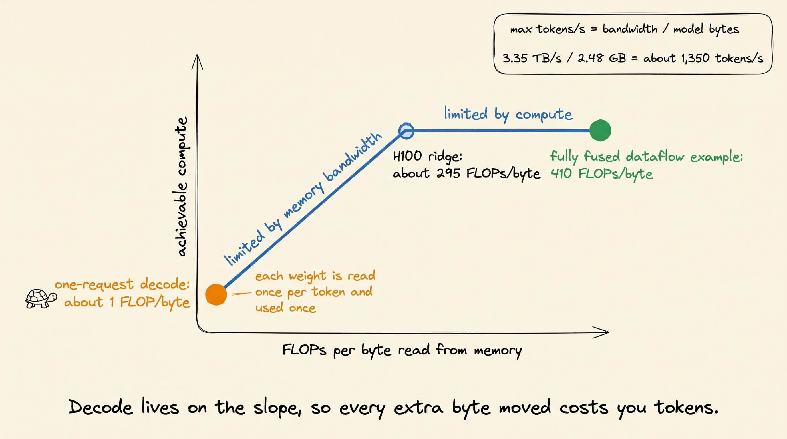
With one request, the model reads every weight once for each new token. That works out to about 1 FLOP of compute for every byte it reads.
An H100 SXM can do about 989 trillion BF16 FLOPs per second, but its HBM delivers only 3.35 TB/s. So decode sits about 300x below the point where compute power becomes the limit.
This gives one request a hard speed ceiling, as the formula below shows:
tokens/s <= memory bandwidth / bytes of weights

H100, GLM-5.3 in BF16, ~40B active:

3.35e12 / (40e9 * 2) = ~42 tokens/s
The same calculation gives 1,351 tokens/s for Llama-3.2-1B and 209 for an 8B model.
The chart below shows how far decode sits from the compute limit:
Kernel boundaries and issues with fusion
Each GPU kernel handles one or a few operations, such as RMSNorm, attention, or the MLP.
Stanford Hazy Research found that vLLM and SGLang use at most 50% of an H100’s bandwidth on Llama-3.2-1B.
At each boundary, the next kernel waits for the last one to finish, then stalls while its weights load from HBM.
The visual below shows these gaps between kernels:
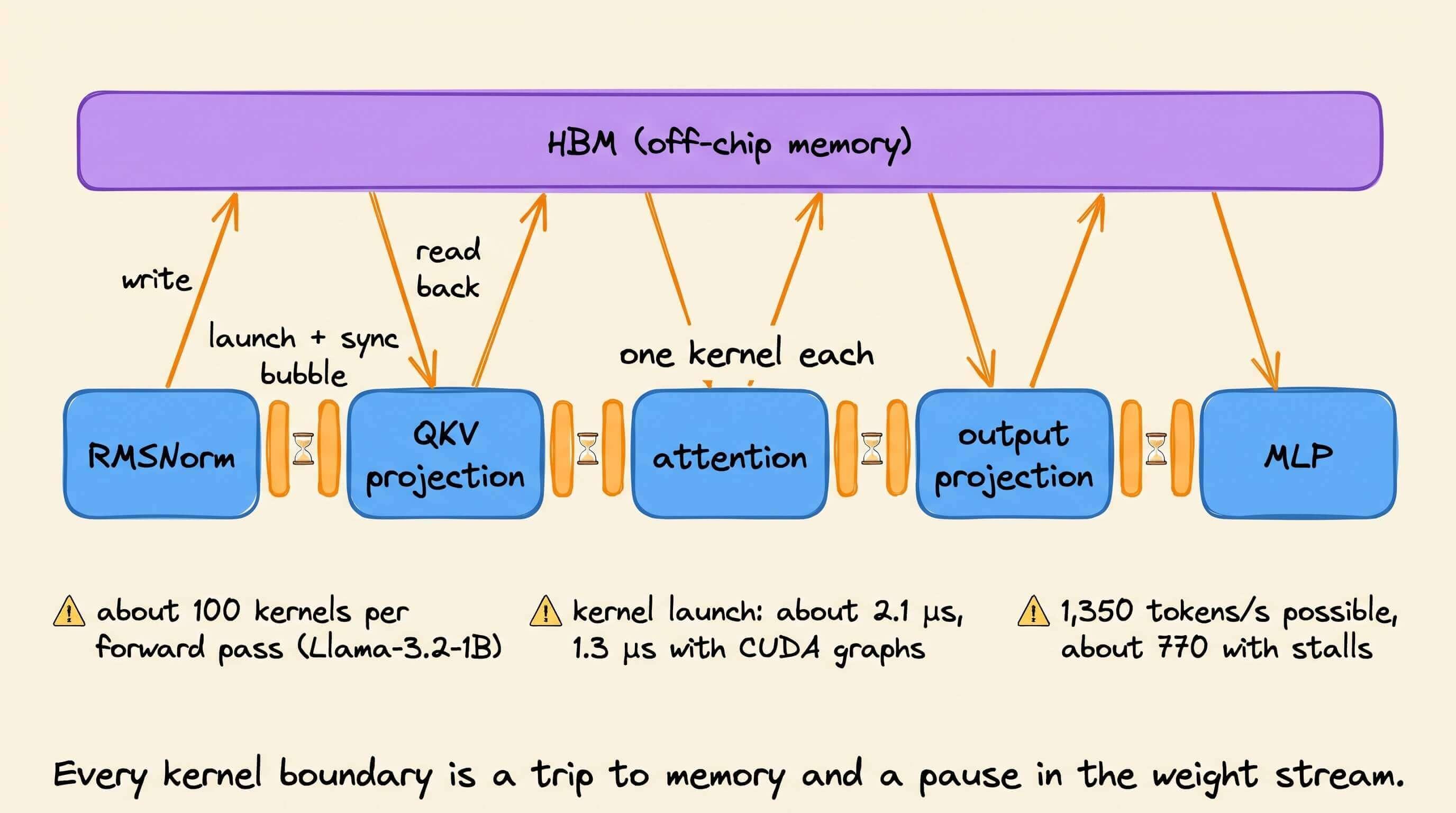
Kernel fusion, which merges several operations into one kernel, is the standard fix. Hazy’s hand-built megakernel fused the whole 1B forward pass this way and reached 78% of bandwidth.
GPU fusion still stops at a few operations. Large intermediate results spill out of the small on-chip SRAM, and the programming model cannot run back-to-back operations as a pipeline.
Dataflow execution and memory tiers on an RDU
An RDU, or Reconfigurable Dataflow Unit, is SambaNova’s AI chip.
Unlike a GPU, it doesn’t run a model one kernel at a time. Instead, its compiler spreads the steps of a decoder layer across the chip, so every step runs in its own spot.
Here’s how that differs from a GPU:
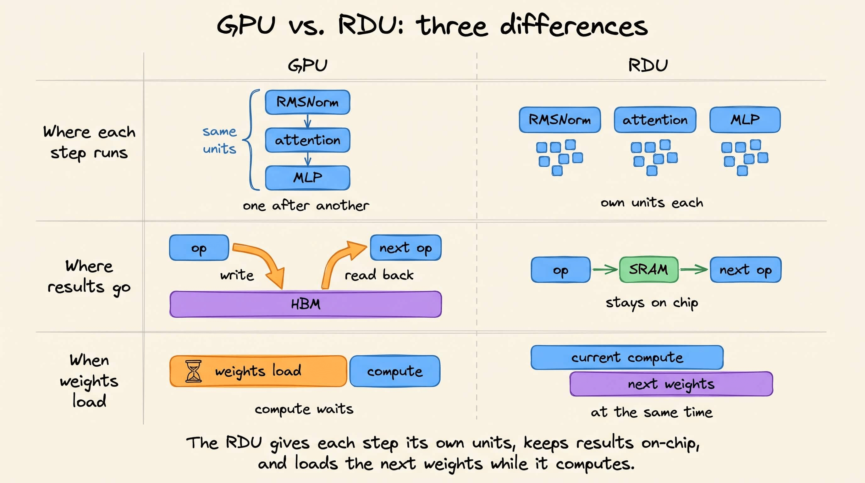
A GPU runs RMSNorm, then attention, then the MLP, one after another. The RDU gives each of these operations its own group of compute units on the chip.
On a GPU, each kernel writes its output to HBM and the next one reads it back. On the RDU, each result passes straight to the next group through on-chip SRAM, so it never leaves the chip.
A GPU kernel stalls while its weights load from HBM. The RDU loads the next step’s weights while the current step is still computing, so no step waits.
Here’s how this layout looks on the chip:
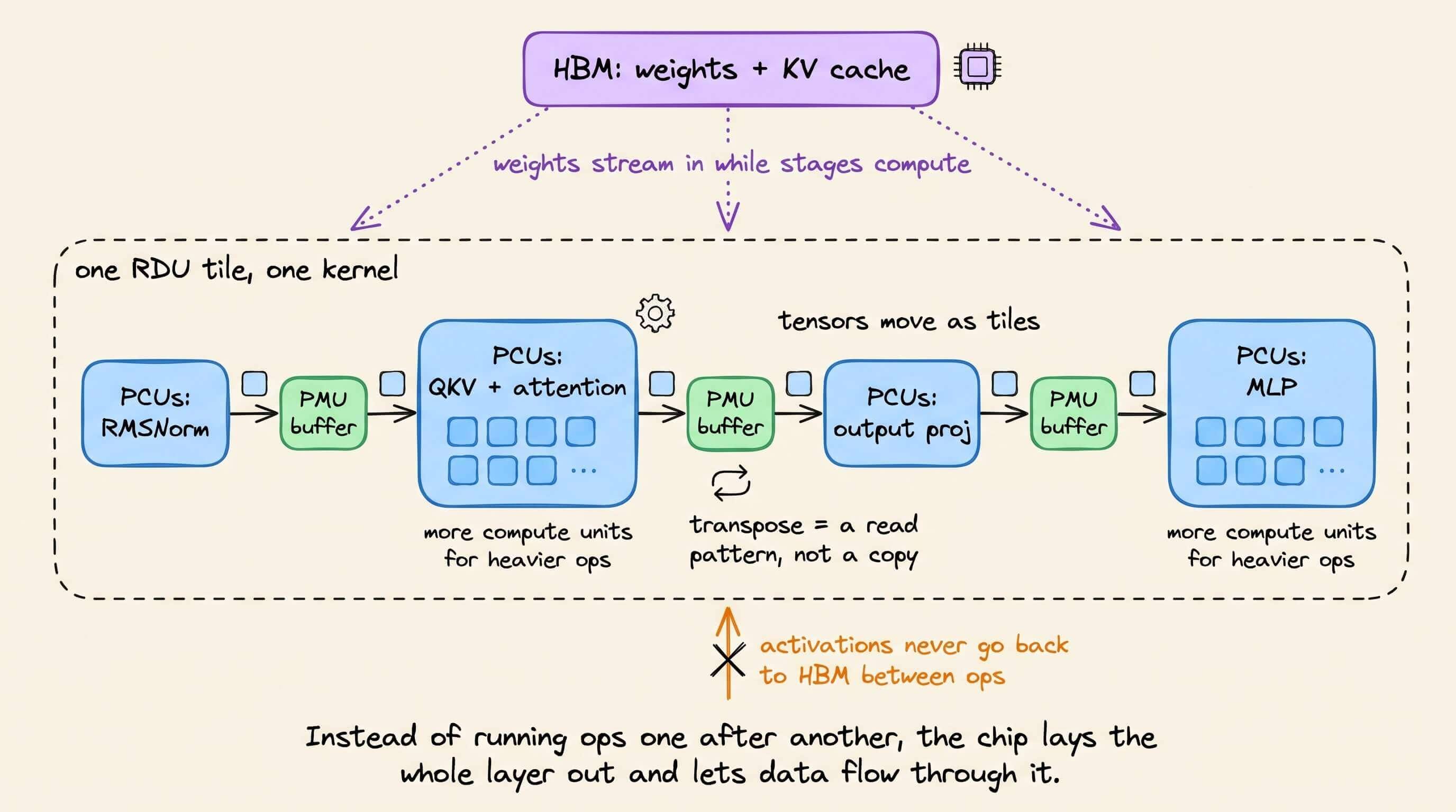
The RDU keeps data in three memory tiers. On-chip SRAM holds activations, 64 GB of HBM holds active weights and KV cache, and up to 512 GB of DDR holds other models.
That DDR sits on the chip itself, so the RDU can switch models without going through the host CPU’s memory.
Whole-decoder kernels and loop conversion
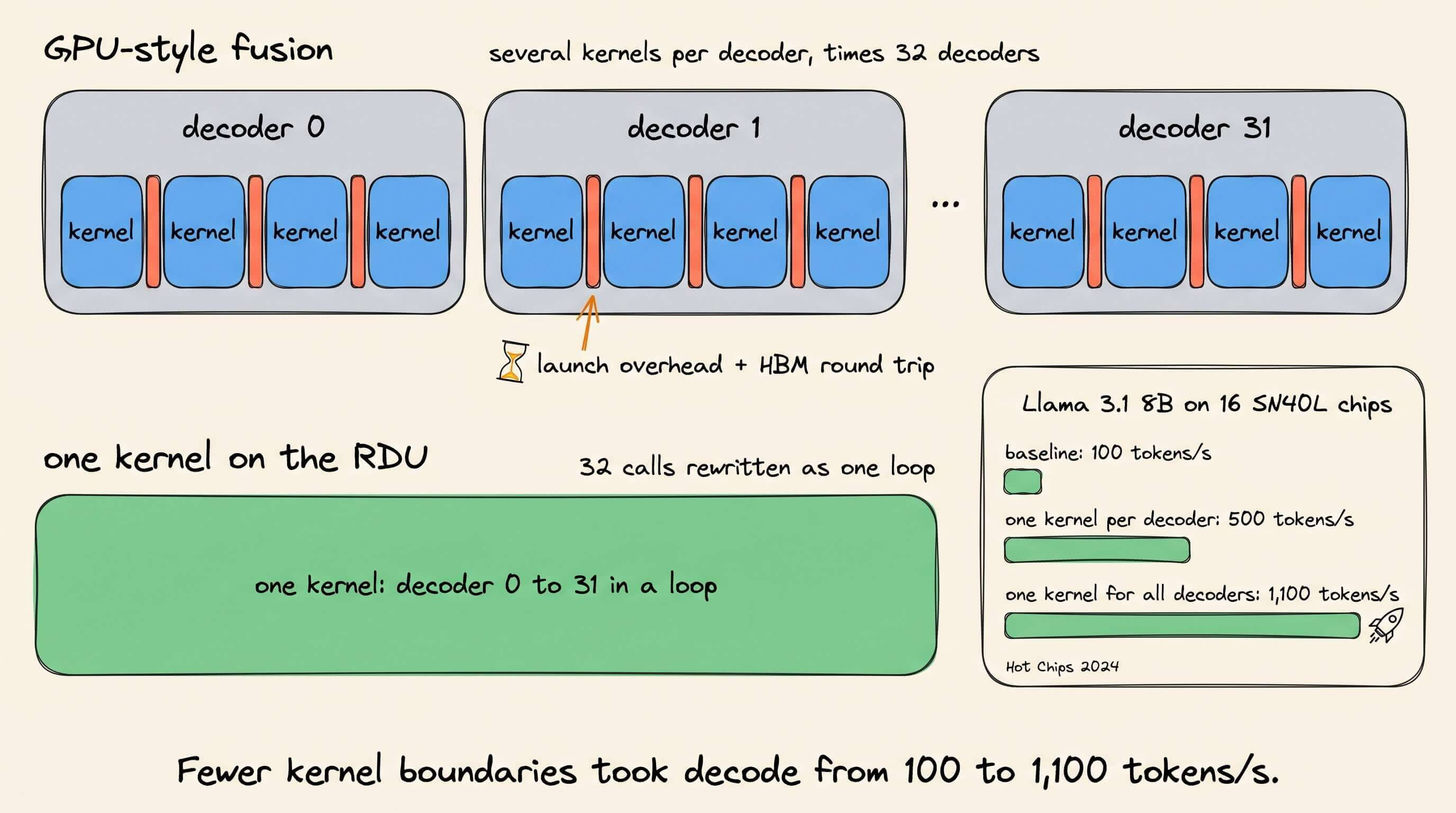
SambaNova applied this to Llama 3.1 8B, which has 32 identical decoder layers. The RDU runs each whole layer as one kernel call, and a compiler pass called loop conversion folds the 32 calls into one loop.
On 16 SN40L chips, the baseline ran at 100 tokens/s. The single-kernel decoder reached 500, and loop conversion reached 1,100.
The visual below compares the GPU and RDU layouts:
Per the SN40L paper, HBM bandwidth then goes only to weights and KV cache, and loading weights during compute uses over 85% of it.
Multi-chip dataflow through the AGCU
A model like GLM-5.3 does not fit on one chip, so its 753B parameters are split across many. Every token then has to move data from chip to chip, and that movement often costs more time than the math.
On a GPU cluster, each GPU writes its result to memory, sends it over the network to the next GPU, and the next GPU reads it back. Each hop adds a wait.
SambaNova’s RDU handles this with the AGCU (Address Generation and Coalescing Unit). The AGCU streams data directly from one RDU to the next, so the dataflow pipeline from the previous section keeps running across chips instead of stopping at every boundary, as shown below.
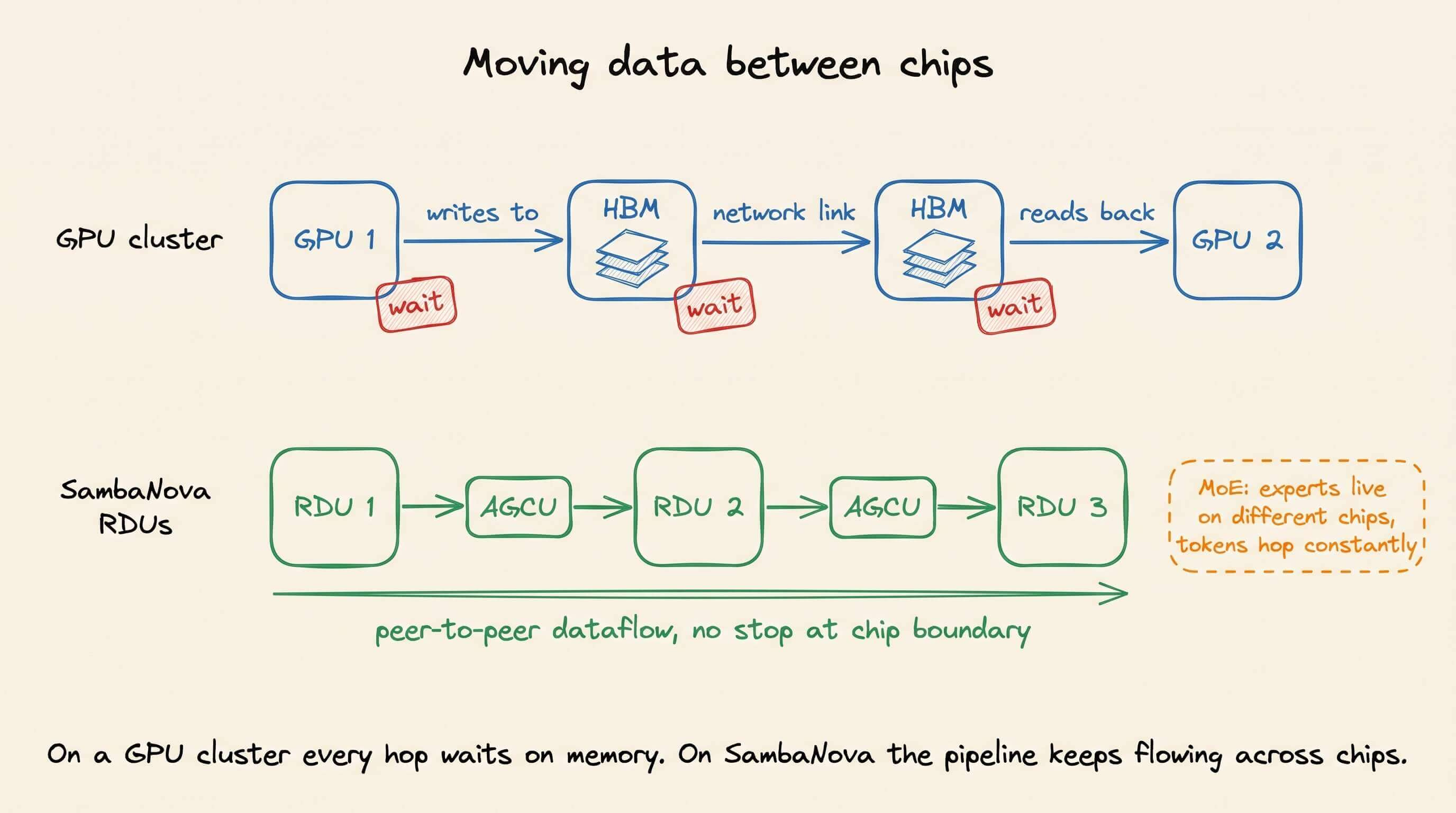
This matters even more for Mixture-of-Experts models. GLM-5.3 activates only about 40B parameters per token, spread across experts on different chips, so tokens hop between chips all the time.
Measuring decode speed on SambaNova Cloud
SambaNova Cloud has an OpenAI-compatible API, so the OpenAI SDK works with a different base URL. The script below streams one request to GLM-5.3 and prints the server’s own timings:
import os
from openai import OpenAI

client = OpenAI(base_url="https://api.sambanova.ai/v1",
                api_key=os.environ["SAMBANOVA_API_KEY"])

stream = client.chat.completions.create(
    model="GLM-5.3", max_tokens=300, stream=True,
    stream_options={"include_usage": True},
    messages=[{"role": "user", "content": "Explain in about 250 words "
               "why LLM decode is memory-bandwidth bound."}])

u = [c.usage for c in stream if c.usage][0].model_dump()

print(f"prefill: {u['time_to_first_token']:.3f} s")

print(f"decode:  {u['completion_tokens_after_first_per_sec']:.0f} tokens/s")
The screenshot below shows this request, plus a ten-step agent loop built on the same call:
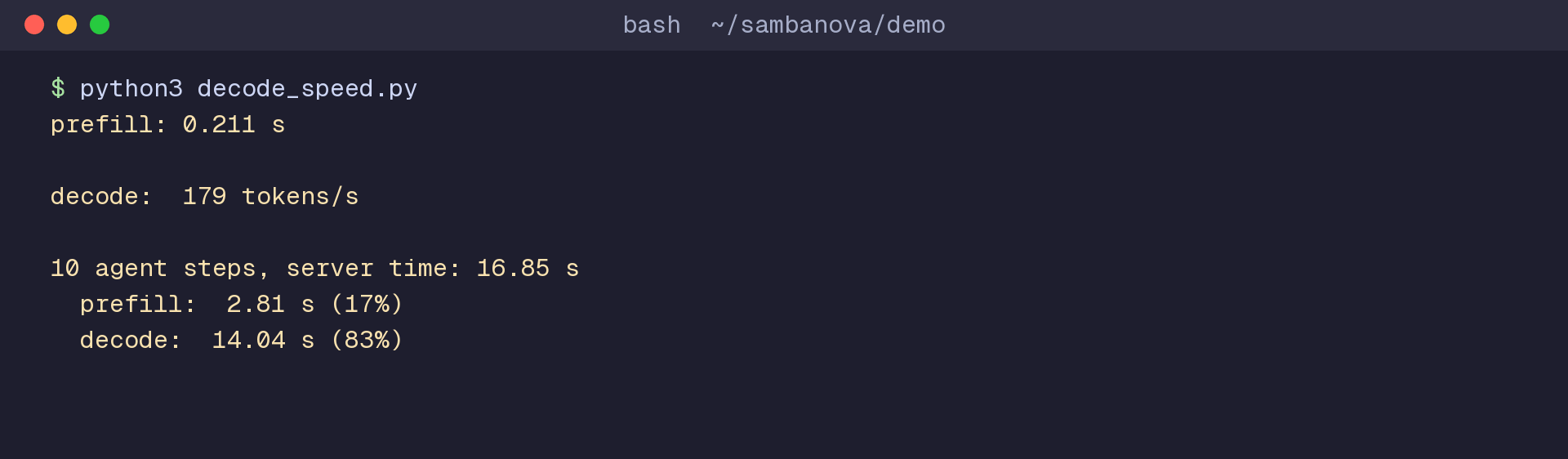
As the screenshot above shows, the run decoded at 179 tokens/s, and prefill finished in 0.211 s.
That is about 4x the ~42 tokens/s ceiling of one H100, since the deployment spreads GLM-5.3’s experts across many chips. In the agent loop, decode took 83% of the 16.85 s of server time.
Disaggregated prefill and decode
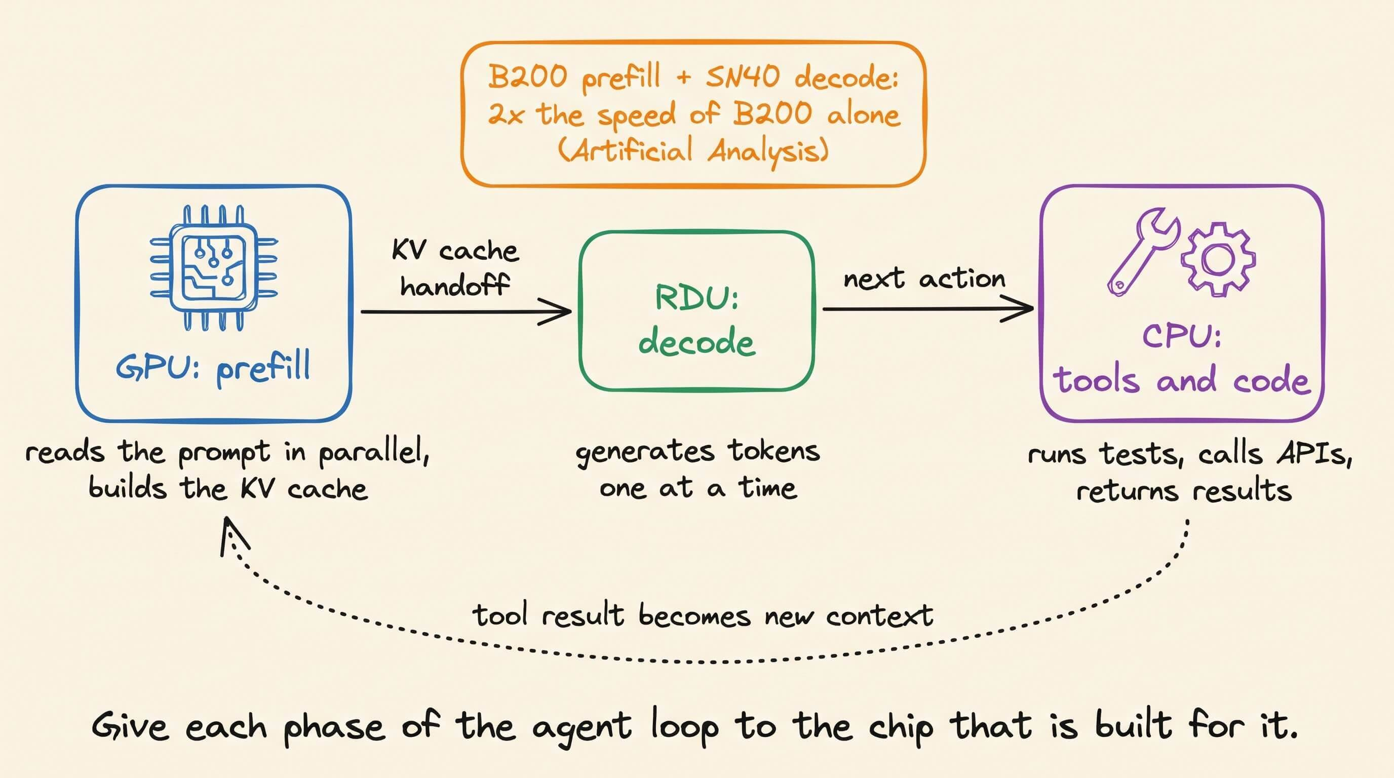
Prefill and decode stress hardware differently, so disaggregated inference runs them on different chips.
In a live demo with an NVIDIA B200 for prefill and an SN40 RDU for decode, SambaNova reported 2x the speed of a B200-only setup, verified by Artificial Analysis.
The visual below shows the split:
Takeaways
Decode with one request is limited by memory bandwidth, and GPU kernel boundaries waste part of it.
A dataflow chip lays the decoder out in space and keeps activations in SRAM, so HBM bandwidth goes to weights and KV cache.
The trade-off is flexibility, since the compiler maps a fixed graph ahead of time.
If your agent is slow, its prefill and decode split is the first thing to measure.
👉 Over to you: what share of your agent’s model time goes to decode?
SambaNova’s page on its dataflow architecture goes deeper here.
If you will be at NeurIPS, you can find SambaNova at the booth in Sydney (December 6-12) and Atlanta (December 8-13), or register for SambaHouse AI Night in Sydney on December 9 here.
Thanks to SambaNova for working with us on this article!
Autoregressive LLMs vs. diffusion LLMs, clearly explained
Generating 500 tokens doesn’t always require 500 sequential decoding steps.
Autoregressive models extend a response one token at a time. Masked diffusion models can predict multiple positions together, then repeat that process to complete the response.
Both can use transformer components such as embeddings, attention, and feed-forward layers. Their attention patterns and training objectives differ.
1) Autoregressive LLMs
In standard autoregressive decoding, each forward pass produces a probability distribution for the next token.
The selected token is appended, and generation continues from that longer sequence.
Causal attention prevents a position from accessing future positions. Earlier token representations therefore stay unchanged as new tokens arrive.
That allows their KV to be cached and reused.
A 500-token response normally requires 500 sequential token-generation steps, although techniques such as speculative decoding can reduce expensive model passes.
2) Diffusion LLMs
In the masked diffusion approach shown below, generation starts with masked output positions alongside the prompt.

A denoising pass predicts candidate tokens for multiple positions using bidirectional context.
With confidence-based sampling, selected predictions are retained while other positions remain masked for subsequent steps.
The model progressively fills the sequence. It doesn’t necessarily produce a complete draft and repeatedly rewrite every token.
Some implementations generate block by block rather than processing the entire response together.
Multiple tokens can be finalized per step, allowing fewer steps than output tokens. The step budget affects both speed and quality.
There are some engineering tradeoffs.
Bidirectional attention makes standard autoregressive KV reuse harder. A token’s representation can change when surrounding positions are updated, even if that token itself stays fixed.
Caching therefore depends on the architecture and decoding strategy. Block diffusion, for example, can support KV caching across completed blocks.
Fewer steps also don’t guarantee lower latency. Each step may process many positions, so total computation and implementation matter.
Bidirectional conditioning also supports filling gaps in text or code.
You can read the diffusion models series here:
👉 Over to you: Where would a diffusion LLM be a better fit than an autoregressive one in your stack?
Good day!