Transform Decision Tree into Matrix Operations.
Make classical ML models deployment friendly.
Inference using a decision tree is an iterative process.
We traverse a decision tree by evaluating the condition at a specific node in a layer until we reach a leaf node.
Today, let me show you a superb technique that allows us to represent inferences from a decision tree in the form of matrix operations.
As a result:
It makes inference much faster as matrix operations can be radically parallelized.
These operations can be loaded on a GPU for even faster inference, making them more deployment-friendly.
Let’s begin!
Below, we only discuss the steps. More intuitive and implementation-specific details are available here: Compiling sklearn models to matrix operations.
Setup
Consider a binary classification dataset with 5 features.
Let’s say we get the following tree structure after fitting a decision tree on the above dataset:
Notations
Before proceeding ahead, let’s assume that:
m → Total features in the dataset (5 in the dataset above).
e → Total evaluation nodes in the tree (4 blue nodes in the tree above).
l → Total leaf nodes in the tree (5 green nodes in the tree).
c → Total classes in the dataset (2 in the dataset above).
Tree to Matrices
The core idea in this conversion is to derive five matrices (A, B, C, D, E) that capture the structure of the decision tree.
Let’s understand them one by one!
Note: The steps we shall be performing below might not make immediate sense so please keep reading. You’ll understand everything once we have derived all 5 matrices.
#1) Matrix A
This matrix captures the relationship between input features and evaluation nodes (blue nodes above).
So it’s an (m×e) shaped matrix.
A specific entry is set to “1” if the corresponding node in the column evaluates the corresponding feature in the row.
For instance, in our decision tree, “Node 0” evaluates “Feature 2”.
Thus, the corresponding entry will be “1” and all other entries will be “0.”
Filling out the entire matrix this way, we get:
#2) Matrix B
The entries of matrix B are the threshold value at each node. Thus, its shape is 1×e.
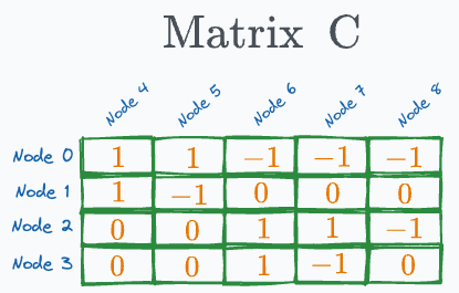
#3) Matrix C
This is a matrix between every pair of leaf nodes and evaluation nodes. Thus, its dimensions are e×l.
A specific entry is set to:
“1” if the corresponding leaf node in the column lies in the left sub-tree of the corresponding evaluation node in the row.
“-1” if the corresponding leaf node in the column lies in the right sub-tree of the corresponding evaluation node in the row.
“0” if the corresponding leaf node and evaluation node have no link.
For instance, in our decision tree, the “leaf node 4” lies on the left sub-tree of both “evaluation node 0” and “evaluation node 1”. Thus, the corresponding values will be 1.
Filling out the entire matrix this way, we get:
#4) Matrix (or Vector) D
The entries of vector D are the sum of non-negative entries in every column of Matrix C:
#5) Matrix E
Finally, this matrix holds the mapping between leaf nodes and their corresponding output labels. Thus, its dimensions are l×c.
If a leaf node classifies a sample to “Class 1”, the corresponding entry will be 1, and the other cell entry will be 0.
For instance, “lead node 4” outputs “Class 1”, thus the corresponding entries for the first row will be (1,0):
We repeat this for all other leaf nodes to get the following matrix as Matrix E:
Done!
With this, we have compiled our decision tree into matrices.
To recall, these are the five matrices we have created so far:
Matrix A captures which input feature was used at each evaluation node.
Matrix B stores the threshold of each evaluation node.
Matrix C captures whether a leaf node lies on the left or right sub-tree of a specific evaluation node or has no relation to it.
Matrix D stores the sum of non-negative entries in every column of Matrix C.
Finally, Matrix E maps from leaf nodes to their class labels.
Inference using matrices
Say this is our input feature vector X (5 dimensions):
The whole inference can now be done using just these matrix operations:
XA < B gives:
The above result multiplied by C gives:
The above result, when matched to D, gives:
Finally, multiplying with E, we get:
The final prediction comes out to be “Class 1,” which is indeed correct!
Notice that we carried out the entire inference process using only matrix operations:
As a result, the inference operation can largely benefit from parallelization and GPU capabilities.
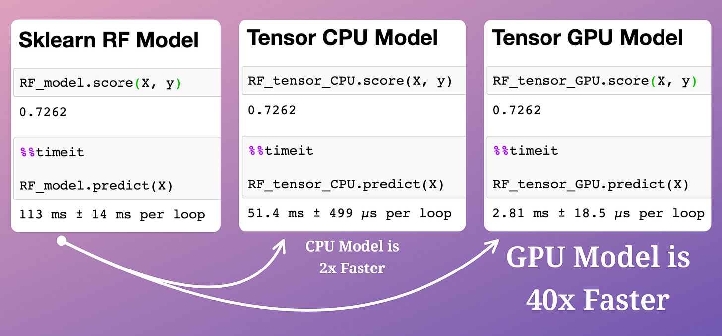
The run-time efficacy of this technique is evident from the image below:
Here, we have trained a random forest model.
The compiled model runs:
Over twice as fast on a CPU (Tensor CPU Model).
~40 times faster on a GPU, which is huge (Tensor GPU Model).
All models have the same accuracy — indicating no loss of information during compilation.
Isn’t that powerful?
To get into more implementation-specific and intuitive details behind the above 5 matrices, we discussed it in detail here: Sklearn Models are Not Deployment Friendly! Supercharge Them With Tensor Computations.
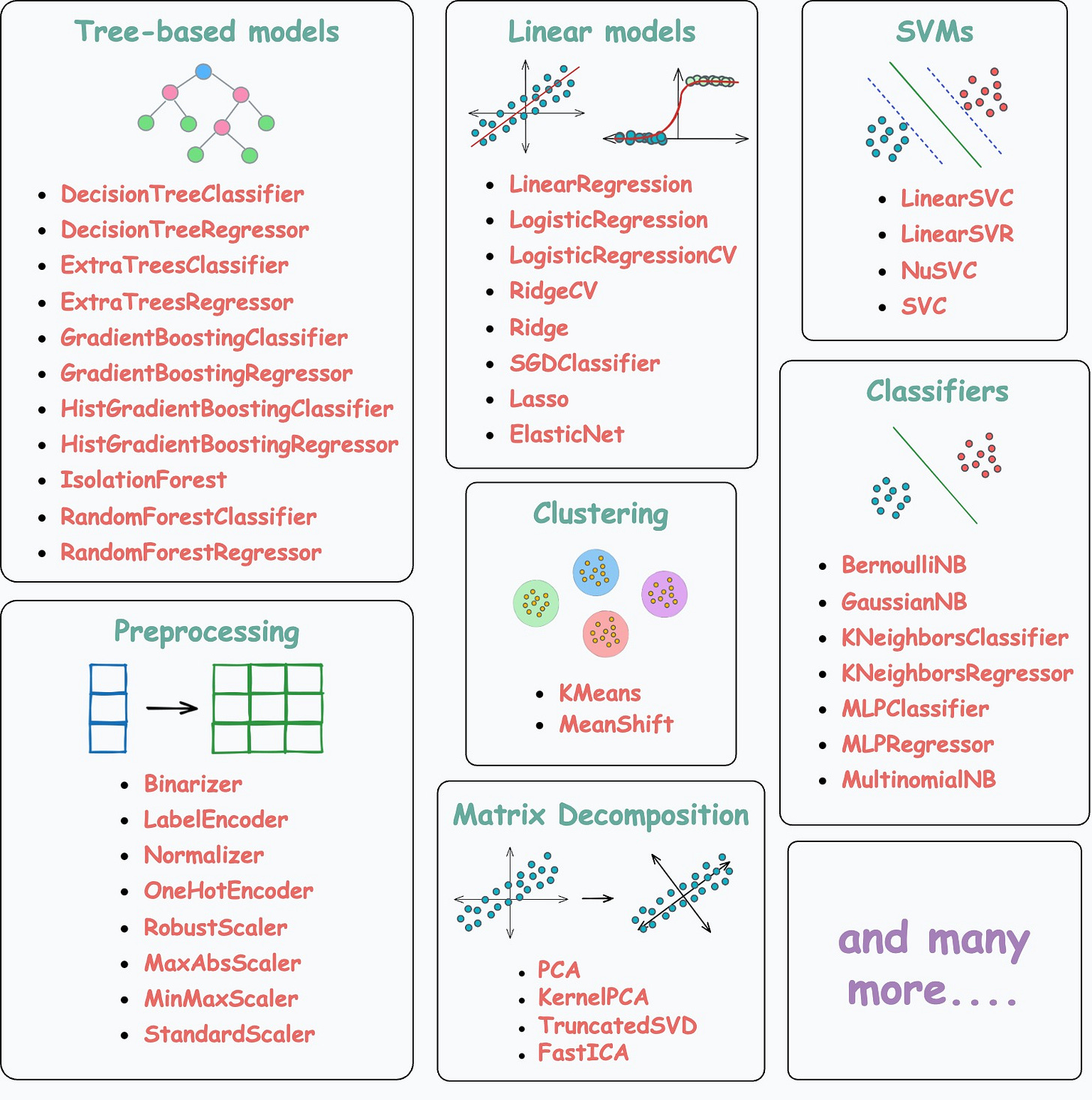
The implementation we discuss does not only apply to tree-based models but all of the following models/encoders/scalers:
Thus, learning about these techniques and utilizing them will be extremely helpful to you in deploying GPU-supported classical ML models.
👉 Over to you: What are some other ways to make classical ML models deployment-friendly?
Thanks for reading!
Whenever you are ready, here’s one more way I can help you:
Every week, I publish 1-2 in-depth deep dives (typically 20+ mins long). Here are some of the latest ones that you will surely like:
[FREE] A Beginner-friendly and Comprehensive Deep Dive on Vector Databases.
A Detailed and Beginner-Friendly Introduction to PyTorch Lightning: The Supercharged PyTorch
You Are Probably Building Inconsistent Classification Models Without Even Realizing
Why Sklearn’s Logistic Regression Has no Learning Rate Hyperparameter?
PyTorch Models Are Not Deployment-Friendly! Supercharge Them With TorchScript.
Federated Learning: A Critical Step Towards Privacy-Preserving Machine Learning.
You Cannot Build Large Data Projects Until You Learn Data Version Control!
To receive all full articles and support the Daily Dose of Data Science, consider subscribing:
👉 If you love reading this newsletter, feel free to share it with friends!
👉 Tell the world what makes this newsletter special for you by leaving a review here :)


Ooo this is cool. Thanks for the demonstration.
Very insightful! Can you give me a pointer to bibliography?