tSNE Projections Can Be Misleading
...and how to avoid being misled.
The performance of the tSNE algorithm (used to visualize high-dimensional datasets) heavily depends on perplexity—a hyperparameter of tSNE.
That is why it is also considered the most important hyperparameter in the tSNE algorithm.
Simply put, the perplexity indicates a rough estimate for the number of neighbors a point may have in a cluster.
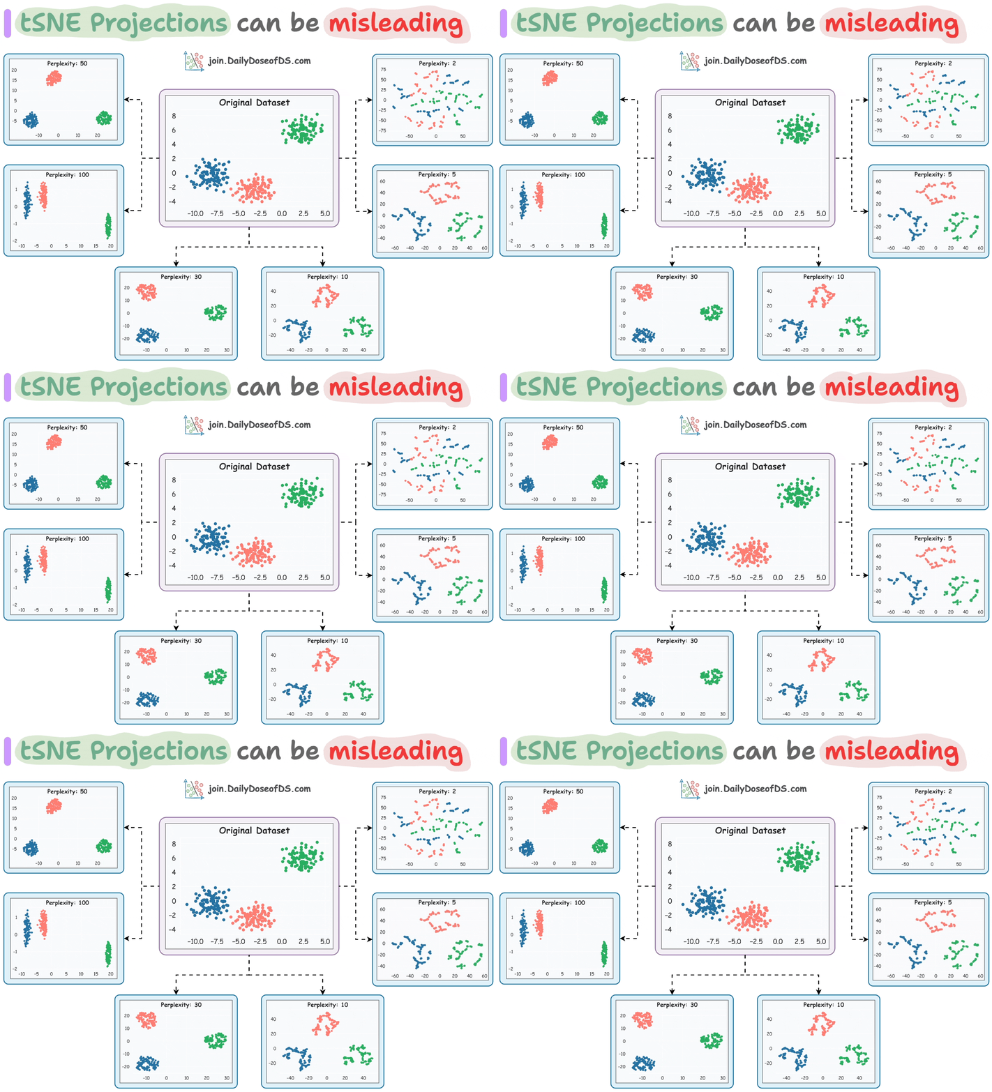
And different values of perplexity create very different low-dimensional clusters, as depicted below:
While most projections depict the original three clusters, they vary significantly in shape.
So here are five key takeaways from the above graphic:
1) Never make any conclusions about the original cluster shape by looking at these projections.
Different projections have different low-dimensional cluster shapes, and they do not resemble the original cluster shape.
Although, in this case, the clusters were color-coded, which provided more clarity. But it may not always be the case since tSNE is an unsupervised algorithm.
2) Cluster sizes in a tSNE plot do not convey anything either.
3) The dimensions (or coordinates of data points) created by tSNE in low dimensions have no inherent meaning.
The axes tick labels of the low-dimensional plots are different and somewhat random.
Similar to PCA’s principal components, they offer little interpretability.
4) The distances between clusters in a projection do not mean anything.
In the original dataset, the blue and red clusters are close.
Yet, most projections do not preserve the global structure.
5) Strange things happen at perplexity=2 and perplexity=100.
At
perplexity=2, the low-dimensional mapping conveys nothing.As discussed earlier, the
perplexityvalue provides a rough estimate of the number of neighbors a point may have in a cluster.tSNE tries to maintain approx. 2 points per cluster. That is why the distortion.
At
perplexity=100, the global structure is preserved, but the local structure gets distorted.
As a concluding note, ideal values typically lie in the range [5,50].
Next time you use tSNE, consider the above points, as these plots can get tricky to interpret.
This is especially true if you don’t understand the internal workings of this algorithm.
Nonetheless, understanding the algorithm will massively help you develop an intuition on its interpretability.
If you are curious to learn more, we have a full 25-minute deep dive on tSNE.
It formulates tSNE from scratch and even implements it from scratch (using NumPy): Formulating and Implementing the tSNE Algorithm From Scratch.
Here’s an intriguing thing we covered.
In the tSNE sklearn documentation, why is the learning rate so high compared to the typical range?
Ever wondered why?
It will become clear once you understand the internal mechanics.
Read here: Formulating and Implementing the tSNE Algorithm From Scratch.
👉 Over to you: What are some other common mistakes people make when using t-SNE?
Here's another "from scratch" formulation and implementation👇
Formulating and Implementing XGBoost From Scratch
If you consider the last decade (or 12-13 years) in ML, neural networks have dominated the narrative in most discussions.
In contrast, tree-based methods tend to be perceived as more straightforward, and as a result, they don't always receive the same level of admiration.
However, in practice, tree-based methods frequently outperform neural networks, particularly in structured data tasks.
This is a well-known fact among Kaggle competitors, where XGBoost has become the tool of choice for top-performing submissions.
One would spend a fraction of the time they would otherwise spend on models like linear/logistic regression, SVMs, etc., to achieve the same performance as XGBoost.
Learn about its internal details by formulating and implementing it from scratch here →
P.S. For those wanting to develop “Industry ML” expertise:
At the end of the day, all businesses care about impact. That’s it!
Can you reduce costs?
Drive revenue?
Can you scale ML models?
Predict trends before they happen?
We have discussed several other topics (with implementations) in the past that align with such topics.
Here are some of them:
Learn sophisticated graph architectures and how to train them on graph data: A Crash Course on Graph Neural Networks – Part 1.
So many real-world NLP systems rely on pairwise context scoring. Learn scalable approaches here: Bi-encoders and Cross-encoders for Sentence Pair Similarity Scoring – Part 1.
Learn techniques to run large models on small devices: Quantization: Optimize ML Models to Run Them on Tiny Hardware.
Learn how to generate prediction intervals or sets with strong statistical guarantees for increasing trust: Conformal Predictions: Build Confidence in Your ML Model’s Predictions.
Learn how to identify causal relationships and answer business questions: A Crash Course on Causality – Part 1
Learn how to scale ML model training: A Practical Guide to Scaling ML Model Training.
Learn techniques to reliably roll out new models in production: 5 Must-Know Ways to Test ML Models in Production (Implementation Included)
Learn how to build privacy-first ML systems: Federated Learning: A Critical Step Towards Privacy-Preserving Machine Learning.
Learn how to compress ML models and reduce costs: Model Compression: A Critical Step Towards Efficient Machine Learning.
All these resources will help you cultivate key skills that businesses and companies care about the most.


