What is Bhattacharyya Distance?

...And how it differs from KL divergence.

Apr 05, 2024

893 people read the 3 deep dives I opened yesterday:

Model Compression: A Critical Step Towards Efficient Machine Learning → Learn how companies save 1000s of dollars in deployment costs.
You Cannot Build Large Data Projects Until You Learn Data Version Control! → Learn how ML projects are made 100% reproducible with code and data versioning.
Why Bagging is So Ridiculously Effective At Variance Reduction? → Learn the mathematical foundation of Bagging, using which, you can build your own Bagging-based models.

Must read if you want to build core ML skills in a beginner-friendly way. They will remain open for only the next 4 days.

Let’s get to today’s post now.

Assessing the similarity between two probability distributions is quite helpful at times.

For instance, imagine we have a labeled dataset (X, y).

By analyzing the label (y) distribution, we may hypothesize its distribution before building a statistical model.

We also looked at this in a deep dive into generalized linear models (GLMs).

Read it here if you haven’t yet: Generalized Linear Models (GLMs): The Supercharged Linear Regression.

While visual inspection is often helpful, this approach is quite subjective and may lead to misleading conclusions.

Thus, it is essential to be aware of quantitative measures as well.

Bhattacharyya distance is one such reliable measure.

It quantifies the similarity between two probability distributions.

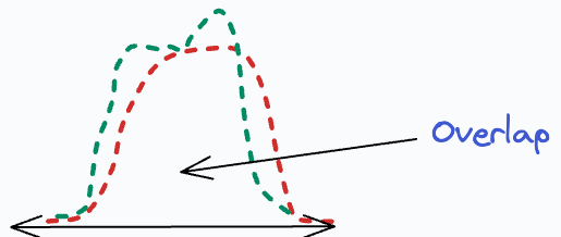
The core idea is to approximate the overlap between two distributions, which measures the “closeness” between the two distributions under consideration.

Bhattacharyya distance between two probability distributions is measured as follows:

For two discrete probability distributions:

Bhattacharyya distance two discrete probability distributions

For two continuous probability distributions (replace summation with an integral):

Bhattacharyya distance two continuous probability distributions

Its effectiveness is evident from the image below.

Here, we have an observed distribution (Blue). Next, we measure its distance from:

Gaussian distribution → 0.19.
Gamma distribution → 0.03.

A high Bhattacharyya distance indicates less overlap or more dissimilarity. This lets us conclude that the observed distribution resembles a Gamma distribution.

Also, the results resonate with visual inspection.

KL Divergence vs. Bhattacharyya distance

Now, many often get confused between KL Divergence and Bhattacharyya distance.

Effectively, both are quantitative measures to determine the “similarity” between two distributions.

However, their notion of “similarity” is entirely different.

The core idea behind KL Divergence is to assess how much information is lost when one distribution is used to approximate another distribution.

The more information is lost, the more the KL Divergence and, consequently, the less the “similarity”.

Also, approximating a distribution Q using P may not be the same as doing the reverse — P using Q.

This makes KL Divergence asymmetric in nature.

Moving on, Bhattacharyya distance measures the overlap between two distributions.

This “overlap” is often interpreted as a measure of closeness (or distance) between the two distributions under consideration.

Thus, Bhattacharyya distance primarily serves a distance metric, like Euclidean, for instance.

Being a distance metric, it is symmetric in nature. We can also verify this from the distance formula:

Just like we use Euclidean distance to report the distance between two points, we can use Bhattacharyya distance to report the distance between two probability distributions.

But if we intend to measure the amount of information lost when we approximate one distribution using another, KL divergence is more apt.

In fact, KL divergence also serves as a loss function in machine learning algorithms at times. Here’s how:

Say we have an observed distribution (P) and want to approximate it with another simpler distribution Q.
So, we can define a simpler parametric distribution Q.
Next, we can measure the information lost by approximating P using Q with KL divergence.
As we want to minimize the information lost, we can use KL divergence as our objective function.
Finally, we can use gradient descent to determine the parameters of Q such that we minimize the KL divergence.

For instance, KL divergence is used as a loss function in the t-SNE algorithm. If you want to learn how, we discussed it here: t-SNE article.

Bhattacharyya distance has many applications, not just in machine learning but in many other domains.

For instance:

Using this distance, we can simplify complex distributions to simple ones if the distance is low.
In image processing, Bhattacharyya distance is often used for image matching. By comparing the color or texture distributions of images, it helps identify similar objects or scenes.
And many more.

The only small caveat is that Bhattacharyya distance does not satisfy the triangle inequality, so that’s something to keep in mind.

👉 Over to you: What other measures do you use in such situations?