

In today’s newsletter:
RAG vs. CAG, explained visually!
What is (was?) GIL in Python?
What is Contrastive Learning?
RAG vs. CAG, explained visually!
RAG is great, but it has a major problem:
Every query hits the vector DB, even for static information that hasn’t changed in months.
This is expensive, slow, and unnecessary.
Cache-Augmented Generation (CAG) fixes this by letting the model keep static information in its key-value (KV) memory, which is what the model builds internally for every token it reads.
And you can take this one step ahead by fusing RAG and CAG as depicted below:
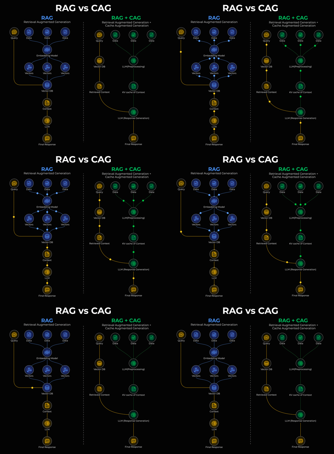
Here’s how it works in simple terms:
In a regular RAG setup, your query goes to the vector database, retrieves relevant chunks, and feeds them to the LLM.
But in RAG + CAG, you divide your knowledge into two layers.
The static, rarely changing data, like company policies or reference guides, gets cached once inside the model’s KV memory.
The dynamic, frequently updated data, like recent customer interactions or live documents, continues to be fetched via retrieval.
This way, you get faster inference, lower costs, and less repeated work.
The trick is being selective about what you cache.
Only cache static, high-value knowledge that rarely changes.
If you cache everything and you’ll hit context limits. separating “cold” (cacheable) and “hot” (retrievable) data keeps this system reliable.
To use this, you can actually start right away since OpenAI and Anthropic already support prompt caching in their APIs.
One thing to know before you scale it.
Prompt caching matches on an exact prefix, byte for byte. So a cached layer only gets reused when it sits at the very front of the context in the same order every time.
So if you:
↳ so reorder two cached policy documents and both turn into a miss
↳ cache document A alone and document B alone, then query both, and the second one misses because the model computed its cached state without ever seeing the first
In production, this looks like a small fraction of your cached blocks serving almost all the hits. The rest just sits there.
The way out comes from how attention behaves. Tokens attend mostly to their own local neighborhood, and only a few reach across document boundaries.
CacheBlend is a technique that recomputes those few and reuses everything else from the separately cached documents.
Multi-document queries run two to four times faster, quality holds, and order stops mattering.
The method is implemented in LMCache, which is fully open source.
GitHub repo: https://github.com/LMCache/LMCache
(don’t forget to star 🌟)
What is (was?) GIL in Python?
For years, the GIL (global interpreter lock) has been the single biggest bottleneck for multi-threaded Python code.
With Python 3.14, you can run Python without the GIL for the first time. Here’s everything you need to know about GIL in Python.
Let’s dive in to learn more today!
Some fundamentals
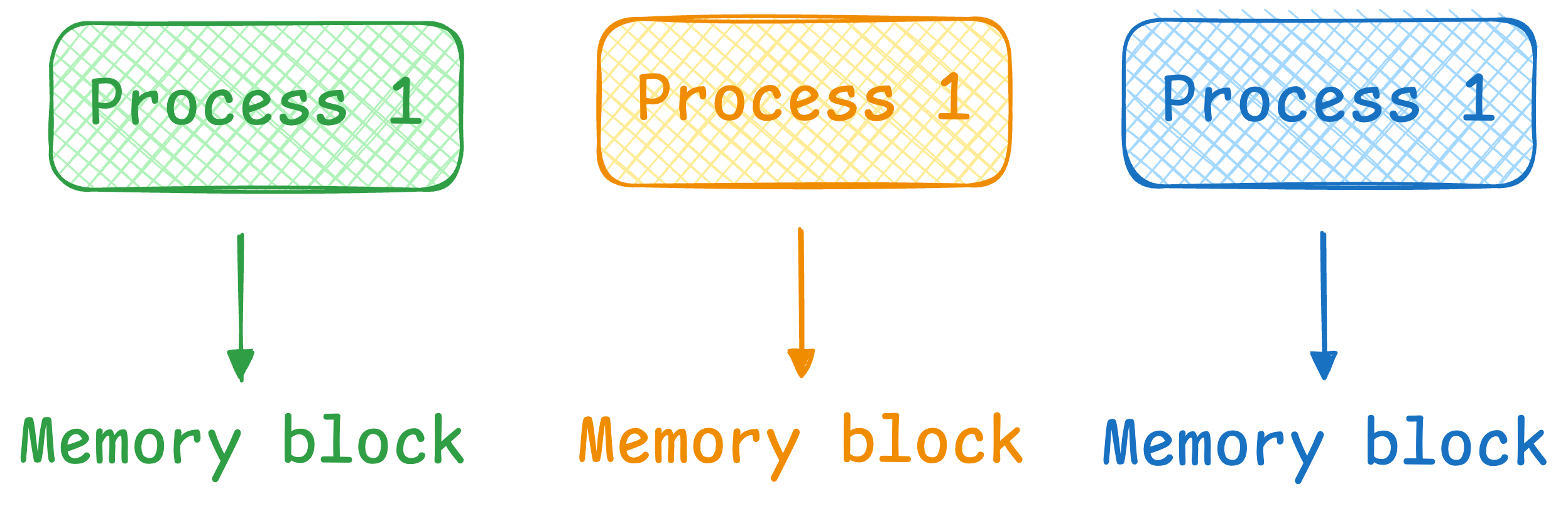
A process is isolated from other processes and operates in its own memory space. This isolation means that if one process crashes, it typically does not affect other processes.
Multi-threading occurs when a single process has multiple threads. These threads share the same resources, like memory.

What is GIL?
Simply put, GIL (global interpreter lock) restricts a process from running more than ONE thread at a time.
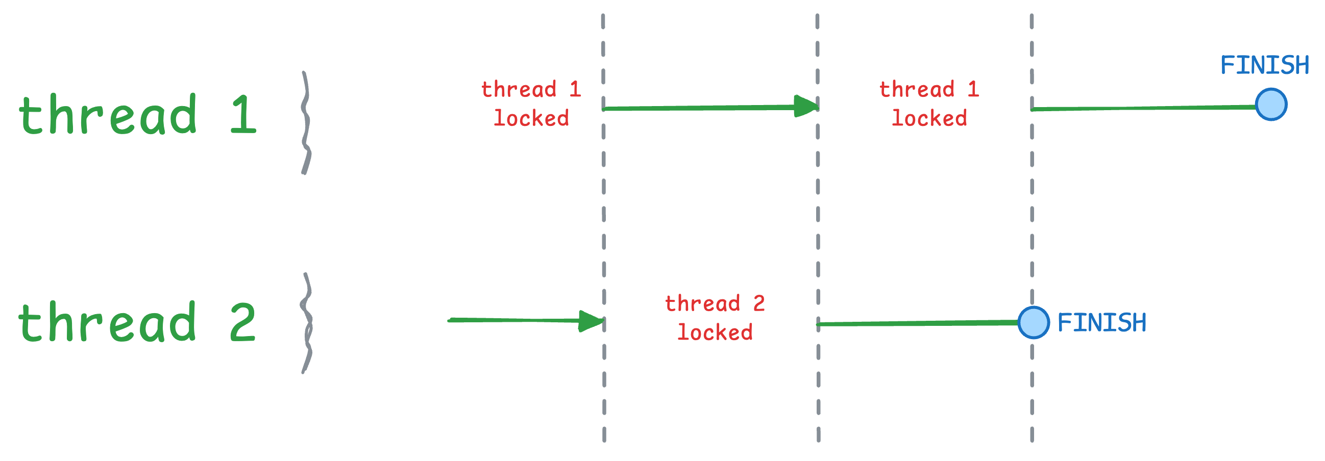
So essentially, a process can have multiple threads, but ONLY ONE can run at a given time.
This means the process cannot use multiple CPU cores for performance optimization, which means multi-threading leads to similar performance as single-threading.
Let’s understand with a code demo!
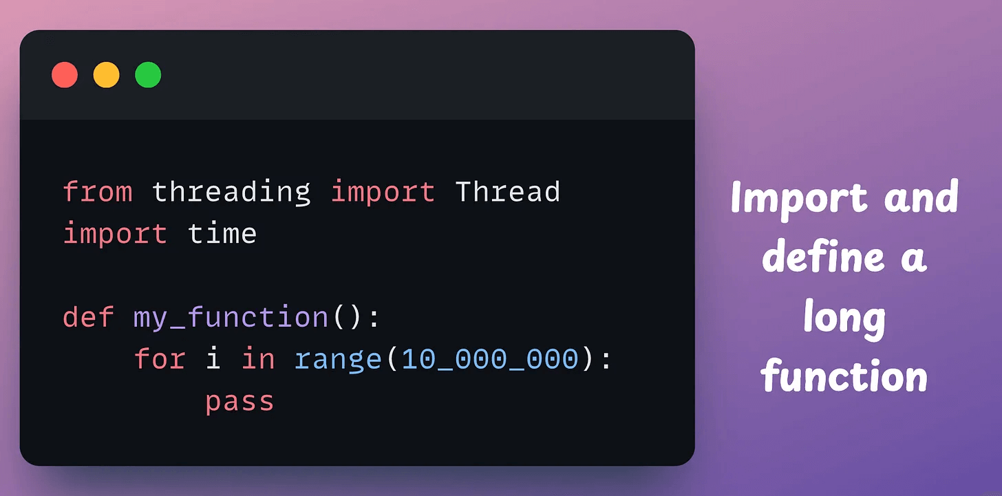
First, we start with some imports and define a long function:
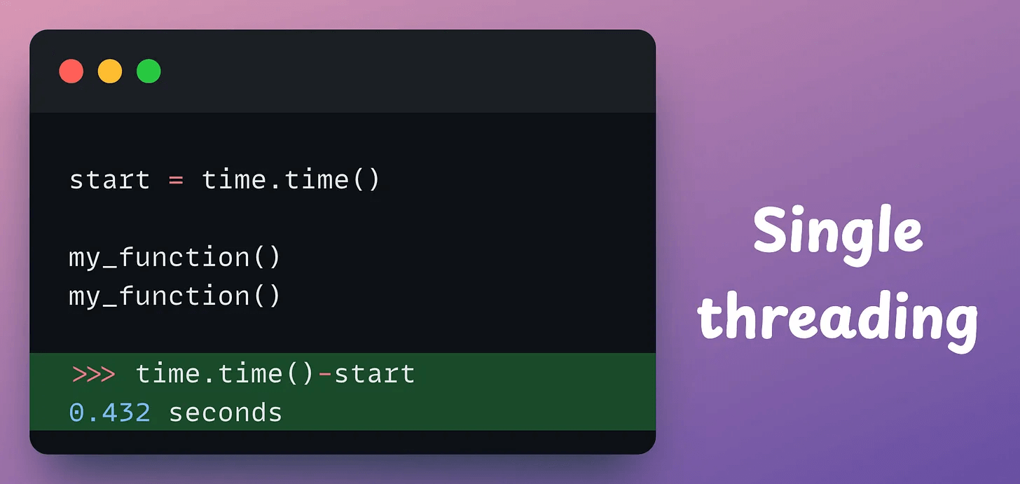
Single threading, wherein we invoke the same function twice, takes 0.432 seconds.
With multi-threading, we create two threads, one for each function, and this takes 0.428 seconds:
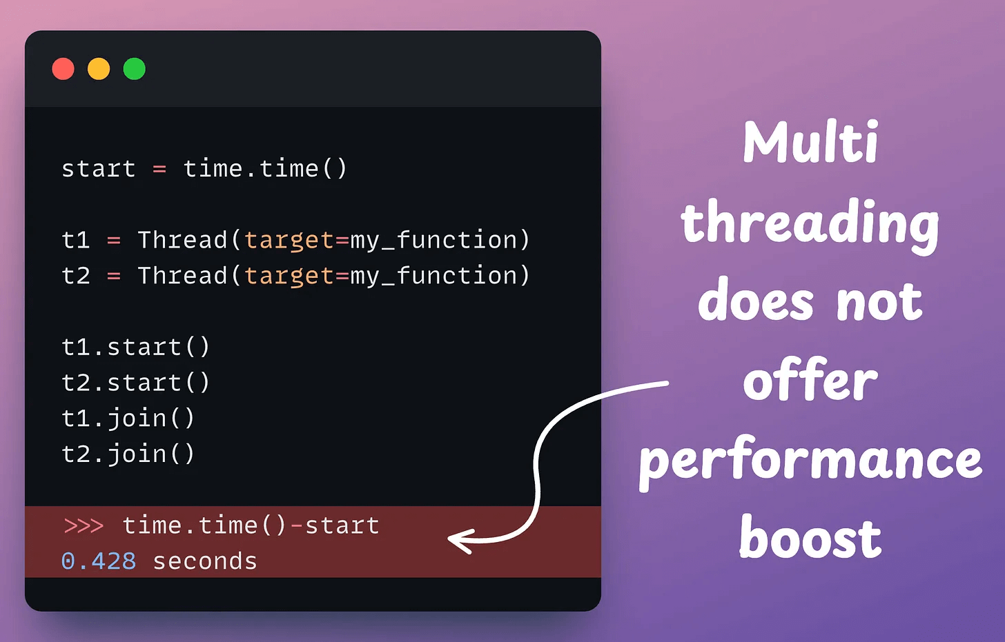
The reason for similar run-time, despite multi-threading, is…
GIL.
On a side note, we do experience a run-time boost with multi-processing:
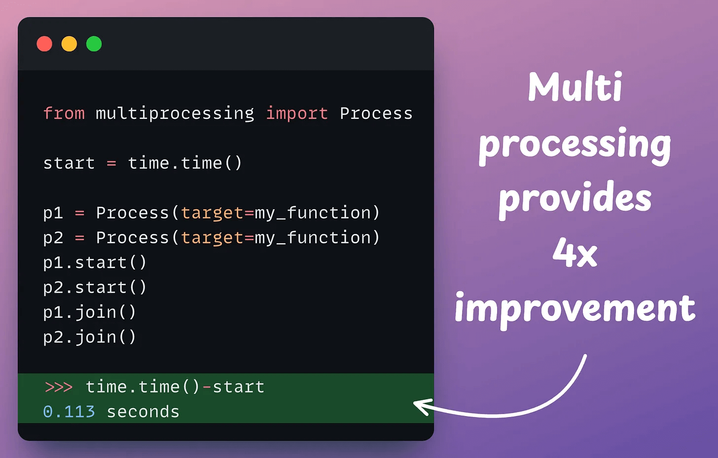
The above three scenarios (single-threading, multi-threading, and multi-processing) can be explained visually as follows:
Single-threading: A single thread executes the same function twice in order:

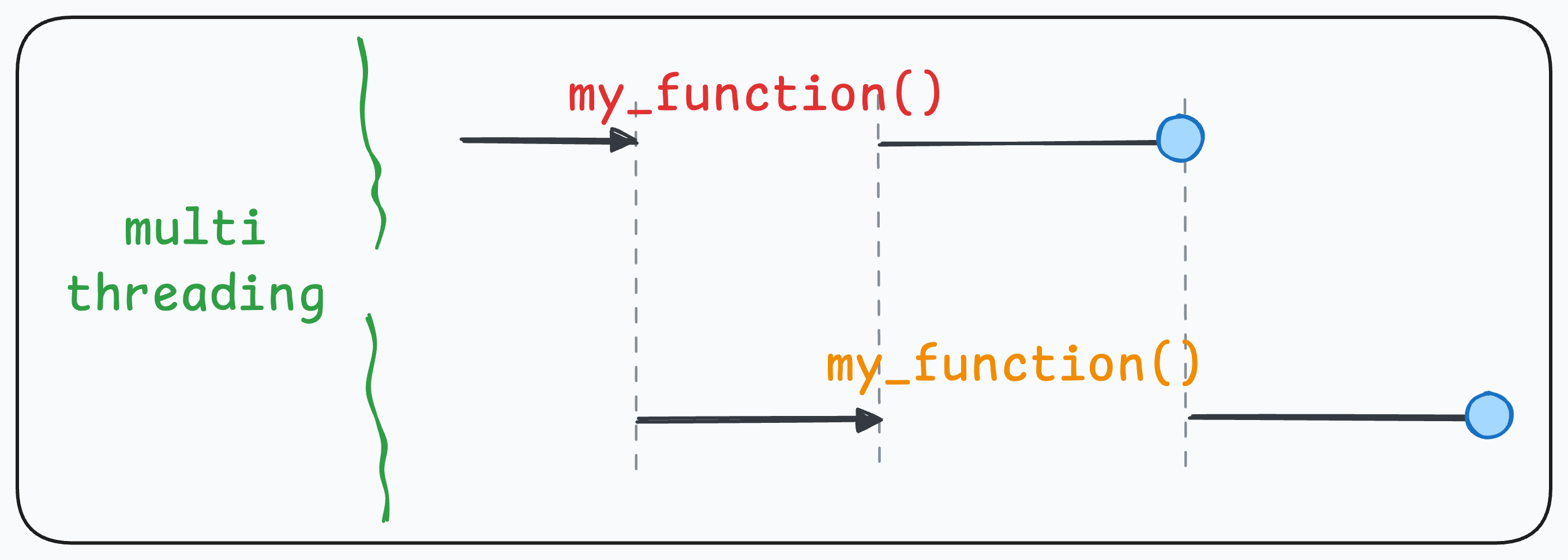
Multi-threading: Each thread is assigned the job to execute the function once. But due to GIL, only one thread can run at a time:
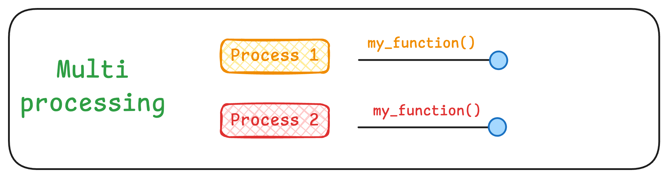
Multi-processing: Each function is executed under a different process:
If this is clear, let’s answer two questions now:
1) Why has Python been using GIL even when it is suboptimal?
Thread safety.
When multiple threads run in a process and share the same resources (such as memory), problems can arise when they try to access and modify the same data.
For instance, say we want to run two operations with two threads on a Python list:

If t1 runs before t2, we get the following output:

If t2 runs before t1, we get the following output:

We get different outputs!
This can lead to race conditions, where the outcome depends on the timing of the threads’ execution.
This, and a few more reasons, made it convenient to execute just one thread at a time.
On a side note, GIL usually affects CPU-bound tasks and not I/O-bound tasks, where multi-threading can still be useful.
2) If multi-processing works, why not use that as a workaround?
This is easier said than done.
Unlike threads, which share the same memory space, processes are isolated.
As a result, they cannot directly share data as threads do.
While there are inter-process communication (IPC) mechanisms like pipes, queues, or shared memory to exchange information between processes, they add a ton of complexity.
Thankfully, Python 3.14 allows us to disable GIL, which means a process can fully utilize all CPU cores.
This video depicts the run-time difference:
We have been testing Python 3.14 lately, and we’ll share these updates in a detailed newsletter issue soon.
That said, if you want to get hands-on with actual GPU programming using CUDA, learn about how CUDA operates GPU’s threads, blocks, grids (with visuals), etc., we covered it here: Implementing (Massively) Parallelized CUDA Programs From Scratch Using CUDA Programming.
👉 Over to you: What are some other reasons for enforcing GIL in Python?
What is Contrastive Learning?
Contrastive Learning is a popular self-supervised learning technique that teaches models to learn useful representations by comparing samples.
Let’s understand more by considering a real-world task.
As an ML engineer, imagine you are responsible for building a face unlock system.
Let’s look through some possible options:
1) Building a Binary classifier
Output 1 if the true user is opening the mobile; 0 otherwise.
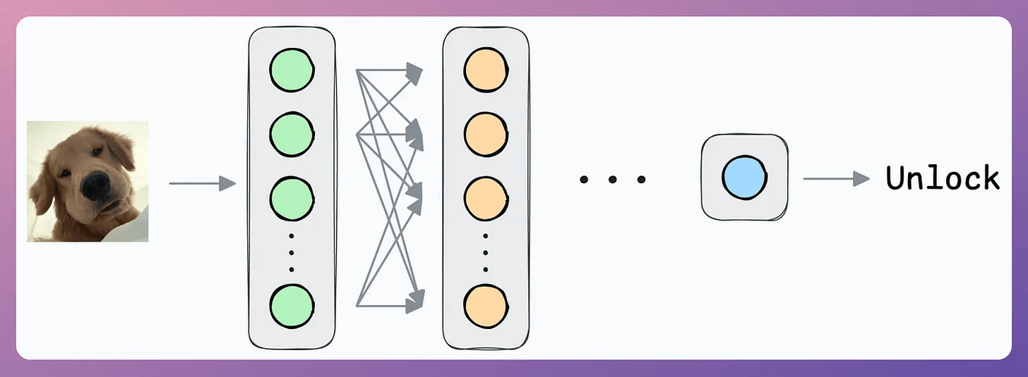
Initially, you can ask the user to input facial data to train the model.
But that’s where you identify the problem.
Their inputs will belong to “Class 1.”
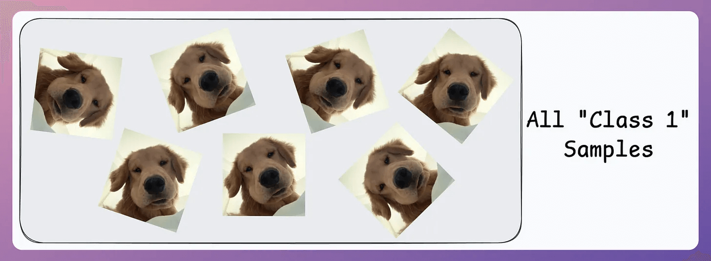
Now, you can’t ask the user to find someone to volunteer for “Class 0” samples since it’s too much hassle for them.
Also, you need diverse “Class 0” samples. Samples from just one or two faces might not be sufficient.
The next possible solution you think of is…
Maybe ship some negative samples (Class 0) to the device to train the model.
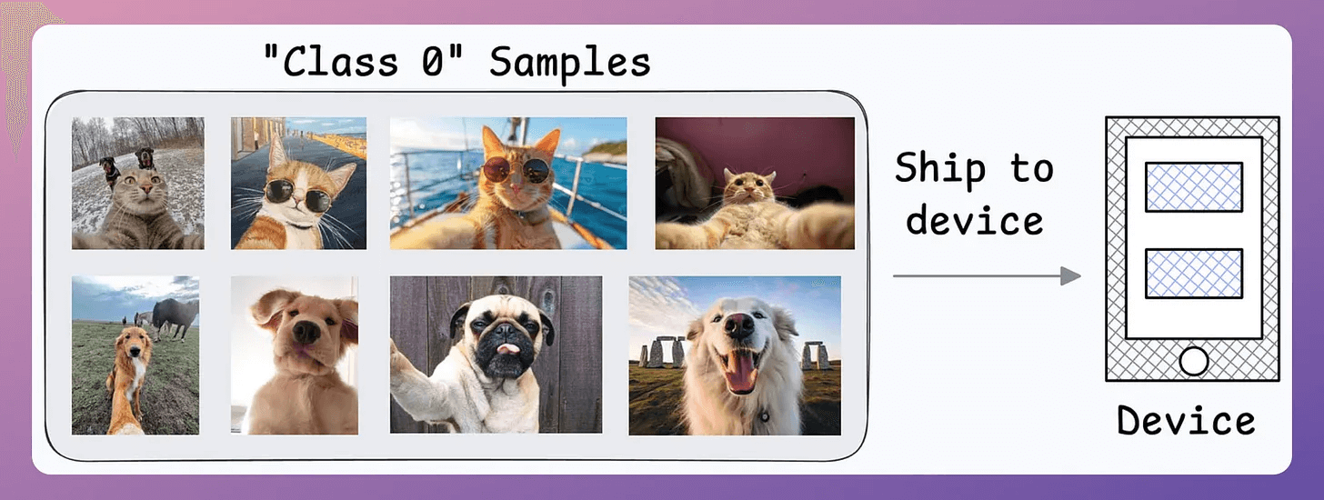
Might work.
But then you realize another problem:
What if another person wants to use the same device?
Since all new samples will belong to the “new face” during adaptation, what if the model forgets the first face?
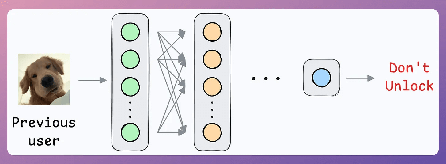
2) How about transfer learning?
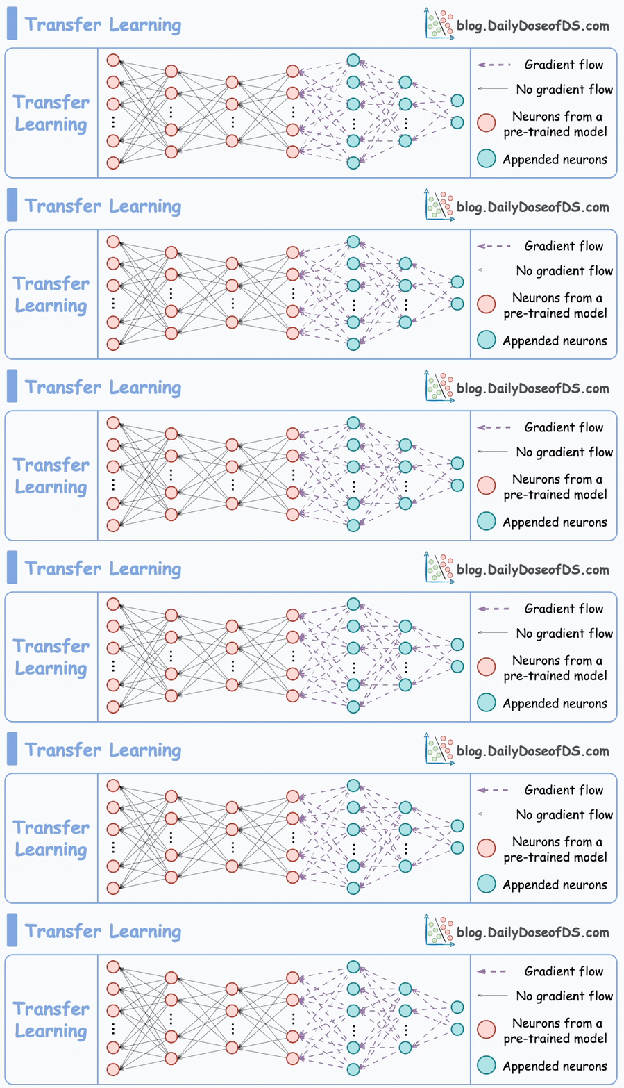
Train a neural network model (base model) on some related task → This will happen before shipping the model to the user’s device.
Next, replace the last few layers of the base model with untrained layers and ship it to the device.
The first few layers would have learned to identify the key facial features, and from there on, training on the user’s face won’t require much data.
But yet again, you realize that you shall run into the same problems you observed with the binary classification model, since the new layers will still be designed to predict 1 or 0.
Solution: Contrastive learning using Siamese Networks
At its core, a Siamese network determines whether two inputs are similar.
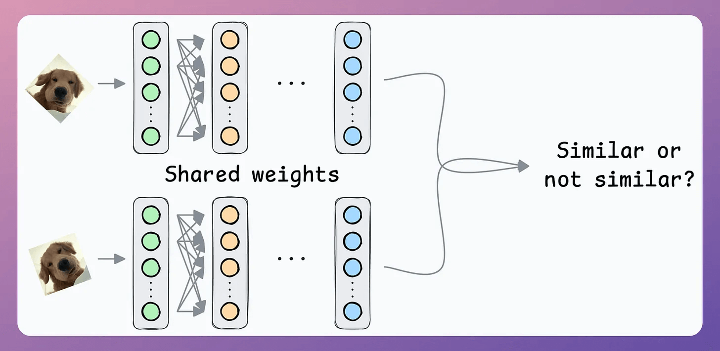
It does this by learning to effectively map both inputs to a shared embedding space (the blue layer above):
If the distance between the embeddings is LOW, they are similar.
If the distance between the embeddings is HIGH, they are dissimilar.
They are beneficial for tasks where the goal is to compare two data points rather than to classify them into predefined categories/classes.
This is how it will work in our case:
Create a dataset of face pairs:
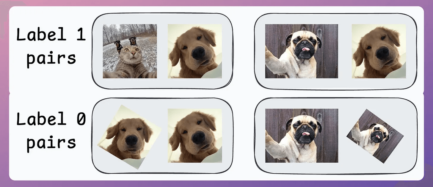
If a pair belongs to the same person, the true label will be 0.
If a pair belongs to different people, the true label will be 1.
After creating this data, define a network like this:
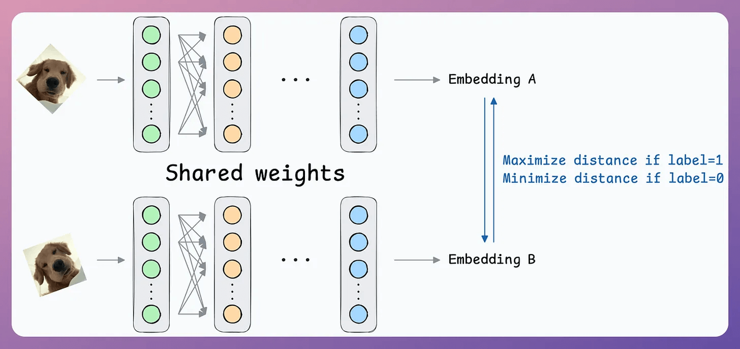
Pass both inputs through the same network to generate two embeddings.
If the true label is 0 (same person) → minimize the distance between the two embeddings.
If the true label is 1 (different person) → maximize the distance between the two embeddings.
Contrastive loss (defined below) helps us train such a model:

where:
yis the true label.Dis the distance between two embeddings.marginis a hyperparameter, typically greater than 1.
Here’s how this particular loss function helps:
When
y=1(different people), the loss will be the following, which will be minimum when D is close to themarginvalue, leading to more distance between the embeddings.

When y=0 (same person), the loss will be the following, which will be minimum when D is close to 0, leading to a low distance between the embeddings.

This way, we can ensure that:
when the inputs are similar, they lie closer in the embedding space.
when the inputs are dissimilar, they lie far in the embedding space.
Siamese Networks in face unlock
Here’s how it will help in the face unlock application.
First, train the model on several image pairs using contrastive loss.
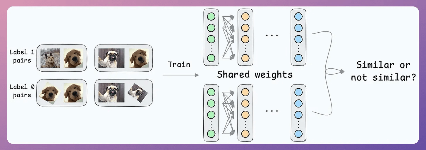
This model (likely after model compression) will be shipped to the user’s device.
During the setup phase, the user will provide facial data, which will create a user embedding:
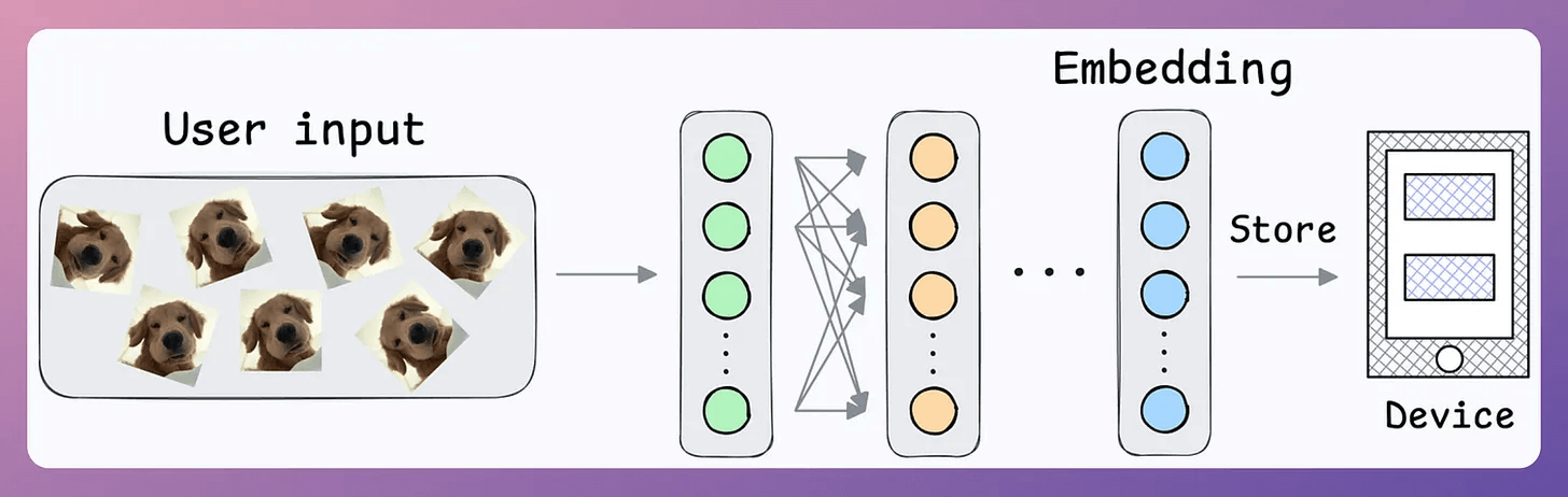
This embedding will be stored in the device’s memory.
Next, when the user wants to unlock the mobile, a new embedding can be generated and compared against the available embedding:
Action: Unlock the mobile if the distance is small.
Done!
Note that no further training was required here, like in the earlier case of binary classification.
Also, what if multiple people want to add their face IDs?
No problem.
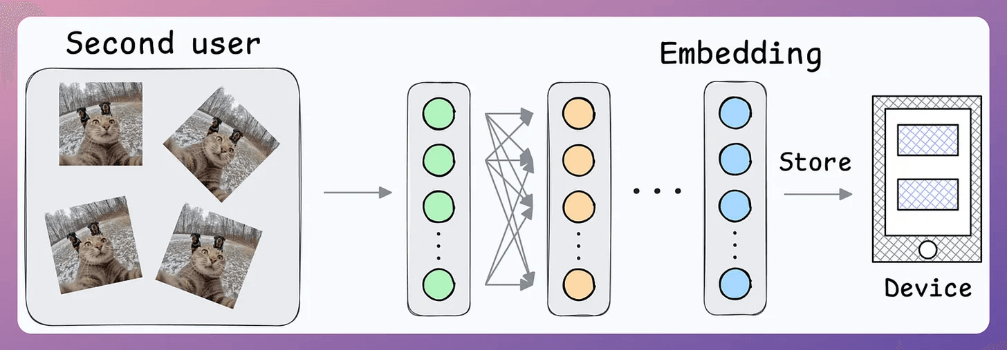
Create another embedding for the new user.
During unlock, compare the incoming user against all stored embeddings.
Here’s some further hands-on reading to learn how to build on-device ML applications:
Learn how to build privacy-first ML systems (with implementations): Federated Learning: A Critical Step Towards Privacy-Preserving Machine Learning.
Learn how to compress ML models and reduce costs: Model Compression: A Critical Step Towards Efficient Machine Learning.
👉 Over to you: Siamese Networks are not the only way to solve this problem. What other architectures can work?
Good day!