What Makes PCA a Misleading Choice for 2D Data Visualization?

...and here's what to replace it with.

PCA, by its very nature, is a dimensionality reduction technique.

Yet, at times, many use PCA for visualizing high-dimensional datasets.

This is done by projecting the given data into two dimensions and visualizing it.

But as we saw in a recent post, 2D visualizations by PCA can be highly misleading.

More specifically, this happens when the first two components of PCA do not explain most of the original variance, as shown below:

Using PCA for 2D visualization is not recommended

Thus, PCA 2D visualizations are only useful if the first two principal components collectively capture most of the original variance.

This is depicted below:

Safe to use PCA for 2D visualization

But in high-dimensional datasets, that might NEVER be true.

So what to do in such cases?

t-SNE is a remarkably better approach for such tasks.

Unlike PCA, t-SNE is specifically meant to create data visualizations in low dimensions.

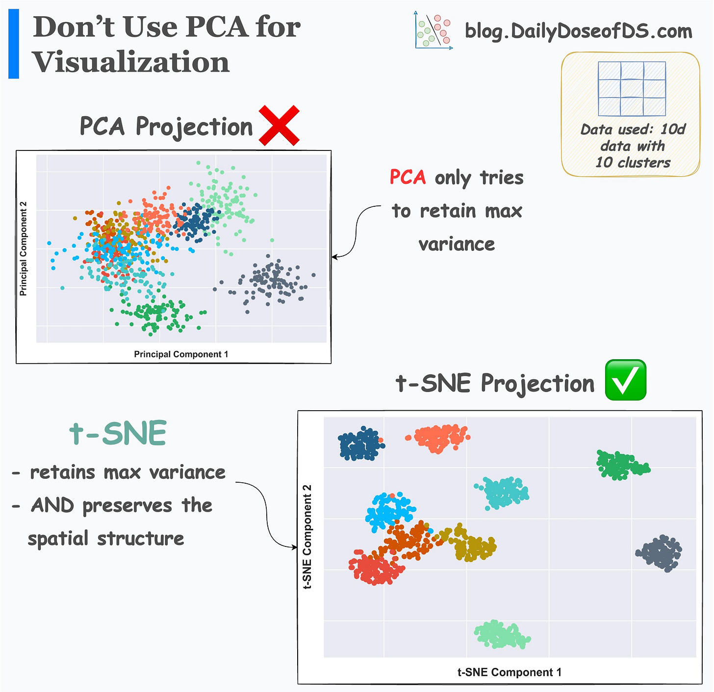
It’s efficacy over PCA is evident from the image below:

PCA vs. t-SNE

• 2D projections created by PCA do not consider local structure. Instead, its principal components primarily focus on preserving the maximum variance. That’s it.

• But t-SNE projections provide much more clarity into data clusters.

• The clusters produced by t-SNE are well separated. But those in PCA have a significant overlap, and they hardly convey anything.

Now, in my experience, most folks have at least heard of the t-SNE algorithm.

They know what it’s used for.

Yet, very few truly understand how it works end-to-end. There are a few questions to ask here:

• How does it so reliably project the high-dimensional datasets to low-dimensions?

• How exactly does it differentiate between a local and global structure in data?

• What is its learning algorithm trying to optimize for?

• When does it not work well?

Can you answer them?

If not, then this is precisely the topic of today’s machine learning deep dive: Formulating and Implementing the t-SNE Algorithm From Scratch.

Formulating and Implementing the t-SNE Algorithm From Scratch

While most folks know about t-SNE, I have seen very few who can explain its internal workings.

In fact, did you know that it was proposed 15 years ago?

Yet, there’s a reason why it continues to be one of the most powerful dimensionality reduction approaches today.

Considering the importance of the topic, today’s article formulates the entire t-SNE algorithm from scratch.

More specifically, the article covers:

• The limitations of PCA.

• The entire end-to-end working of the SNE algorithm (an earlier version of t-SNE).

• What is SNE trying to optimize?

• What are local and global structures?

• Understanding the idea of perplexity visually.

• The limitations of the SNE algorithm.

• How is t-SNE different from SNE?

• Advanced optimization methods used in t-SNE.

• Implementing the entire t-SNE algorithm by only using NumPy.

• A practice Jupyter notebook for you to implement t-SNE yourself.

• Understanding some potential gaps in t-SNE and how to possibly improve it.

• PCA vs. t-SNE comparison.

• Limitations of t-SNE.

• Why is perplexity the most important hyperparameter of t-SNE?

• Important takeaways for using t-SNE.

I know everyone is a fan of visual learning.

Thus, to augment your understanding and ensure that you never forget about it, the article explains every concept visually. Thus, there are (at least) 100 visuals in the entire article.

👉 Interested folks can read it here: Formulating and Implementing the t-SNE Algorithm From Scratch.

Hope you will learn something new today :)

👉 If you liked this post, don’t forget to leave a like ❤️. It helps more people discover this newsletter on Substack and tells me that you appreciate reading these daily insights. The button is located towards the bottom of this email.

Thanks for reading :)