

Get started with all the best tools in the open AI ecosystem for free
The Nebius AI Builder Program launched last week to kickstart developers with $400+ in free credits.
With one free sign-up, developers get credits for Nebius Token Factory, Tavily, Toloka, LangSmith, and more.
Developers also get access to runnable cookbooks and training opportunities from some of the top companies in the industry, providing both the access and the education to get started building on the open AI ecosystem now.
For developers aiming to move into AI engineering or take an existing project beyond demos, the program provides a direct way to build production experience without paying upfront.
Things you’d learn:
Building a deep research agent powered by Tavily and Token Factory.
Build an agent skill for searching for car parts with Kimi K3.
How to use OpenCode with Nebius Token Factory models.
The same learning path would otherwise require several platforms and separate resources.
Join the Nebius AI Builder Program for free at dev.nebius.com/builders and get $400+ in credits and discounts across the stack on day one.
Join early before it runs out.
Thanks to Nebius for partnering today.
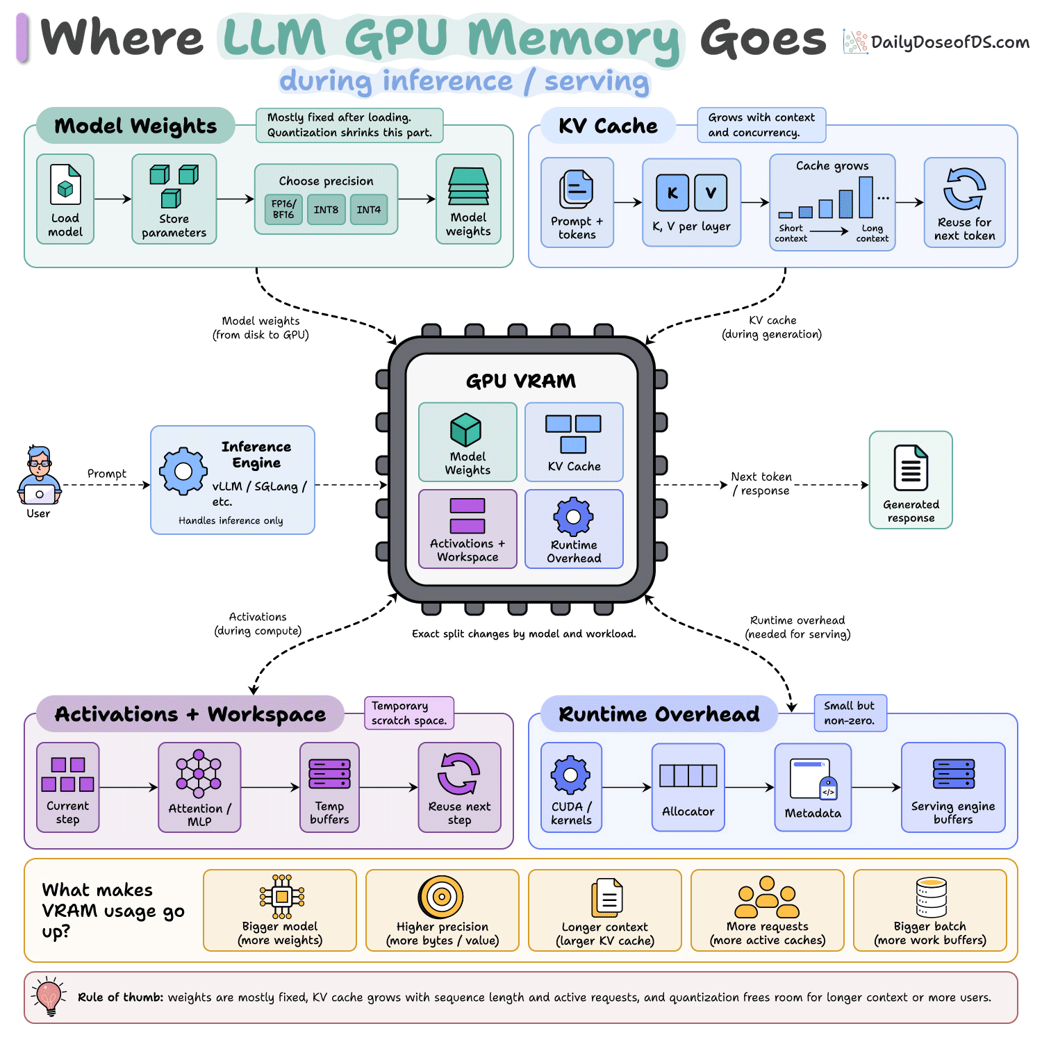
Where does all the VRAM go during LLM inference?
Loading the model is only the first part of the GPU memory story.
Once inference starts, VRAM is divided across model weights, the KV cache, temporary activations and workspace, and runtime overhead. Only one bucket stays roughly fixed. The others change with context length, batch size, concurrency, and model architecture.
This is why “the model fits on the GPU” and “the workload fits on the GPU” are two different statements.
The diagrams below break the memory budget into four useful buckets.
1. Model weights
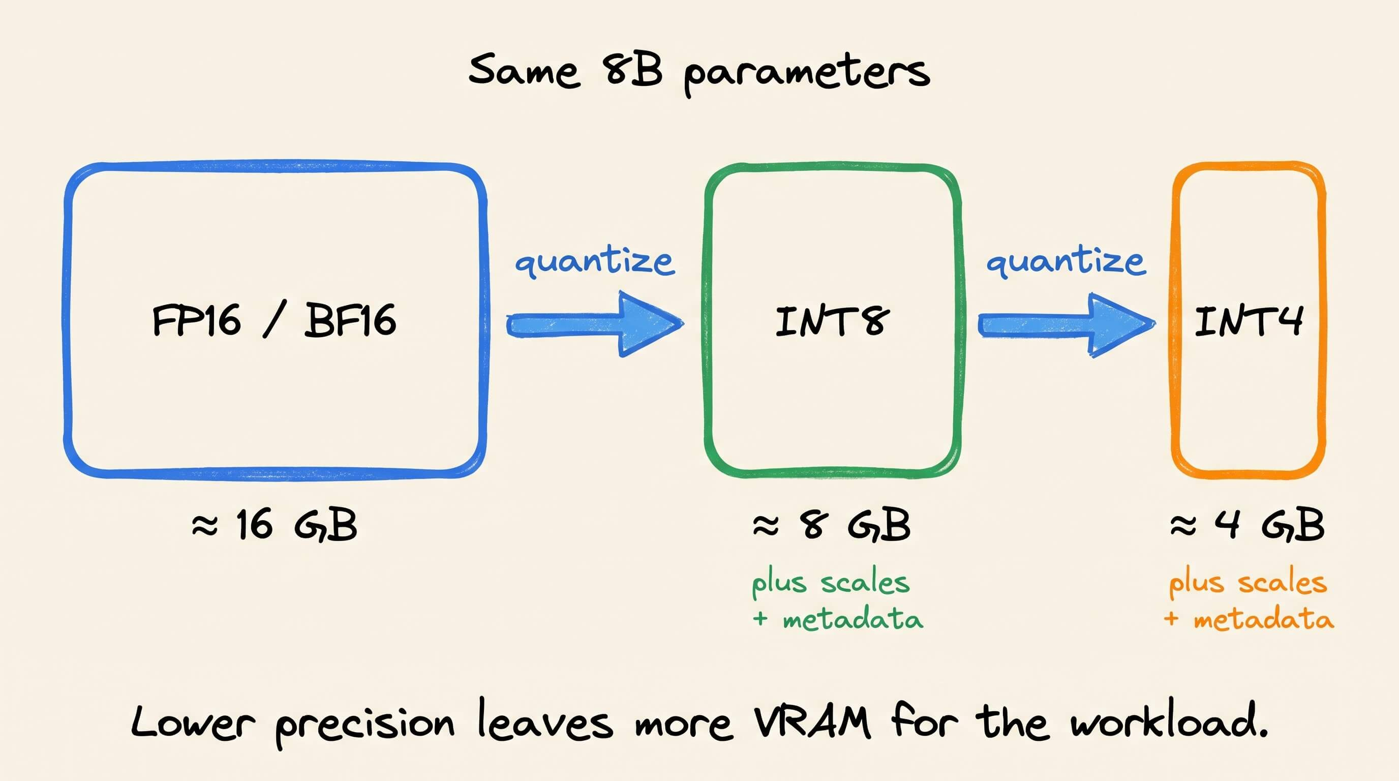
Weights are the mostly fixed part of inference memory. A model with 8 billion parameters needs about 16 GB in FP16 or BF16, 8 GB at 8 bits per parameter, or 4 GB at 4 bits per parameter. Quantized checkpoints also store scales, zero points, and metadata.
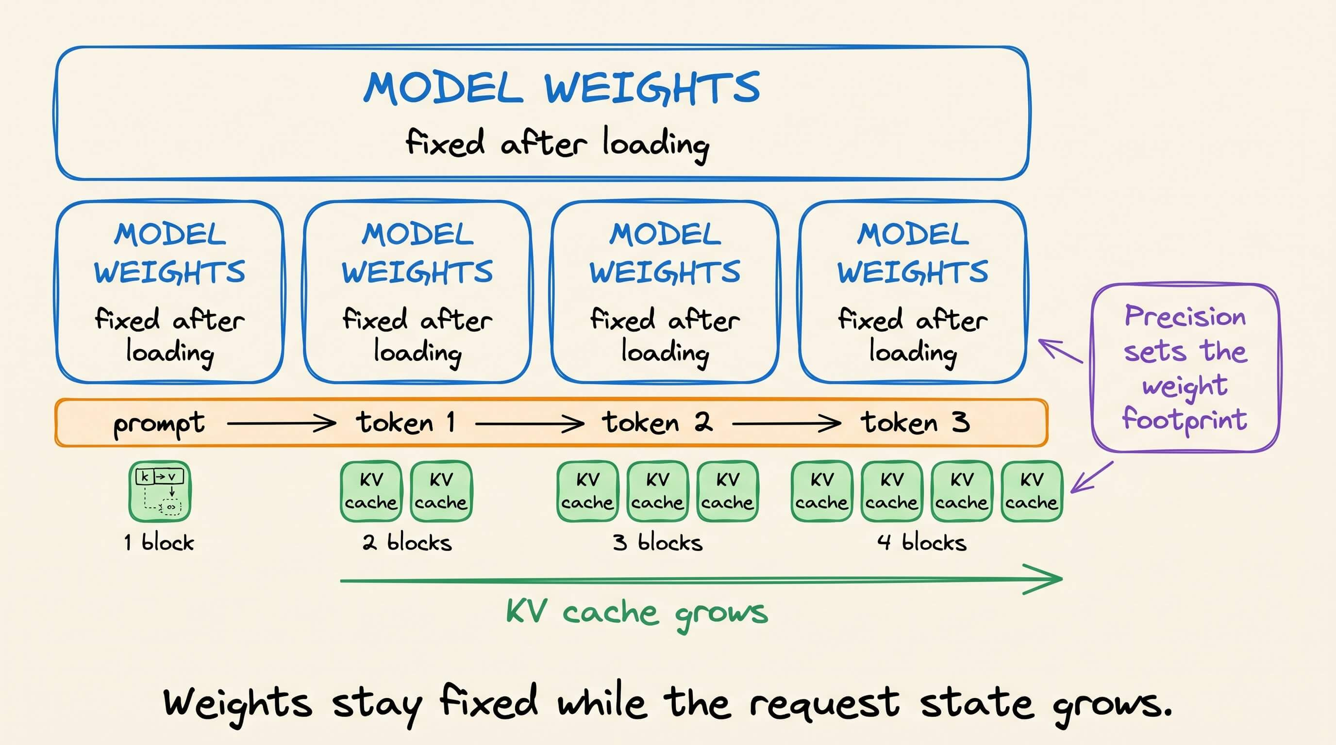
The allocation does not grow during generation. Its main inputs are parameter count, numerical format, and how the model is split across GPUs.
Quantization also creates room for longer contexts, more simultaneous requests, or larger batches. Speed still depends on kernel support and dequantization cost, so lower precision does not guarantee higher throughput.
2. KV cache
The KV cache is the dynamic part that catches many deployments by surprise.
Each transformer layer stores key and value tensors for earlier tokens. During decoding, attention reads them instead of recomputing the full prefix at every step.
The dense-cache approximation below includes the number of active sequences. The factor of two accounts for keys and values. Grouped-query attention reduces this cost because several query heads share fewer KV heads. KV-cache quantization reduces bytes per element, with accuracy and kernel-support tradeoffs.
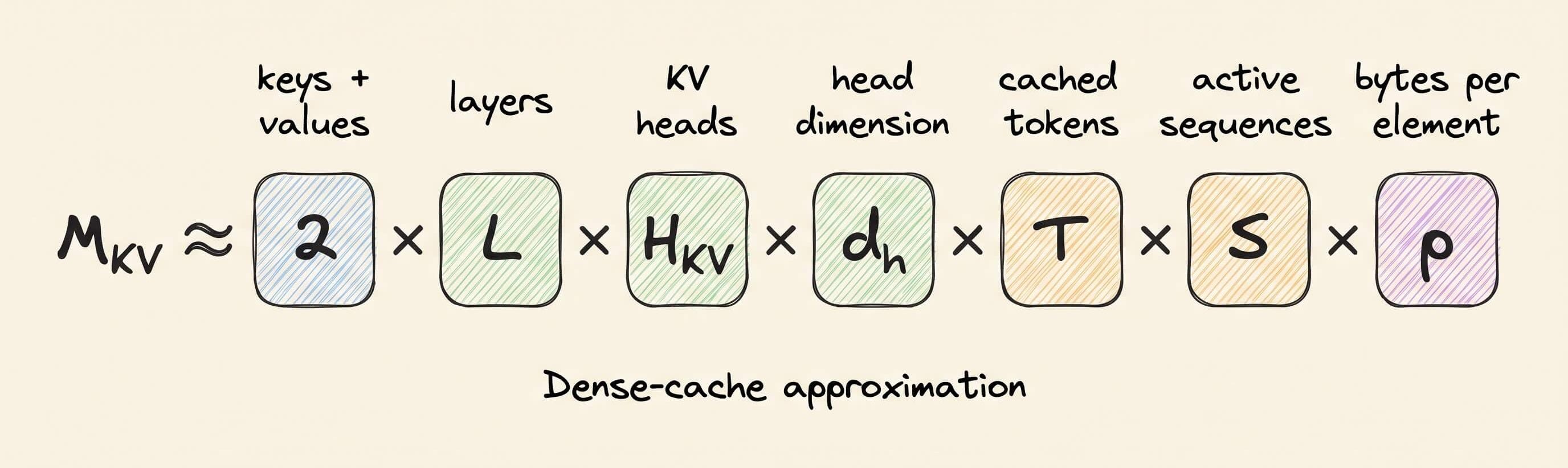
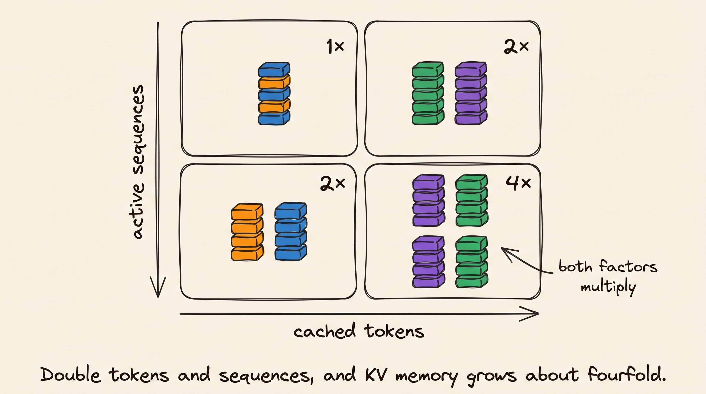
Double the cached tokens and the cache roughly doubles. Double the active sequences and it roughly doubles again. A server handling long conversations can spend more VRAM on KV state than weights.
Serving engines manage this memory in blocks. Paged allocation reduces waste from variable sequence lengths, while prefix caching reuses blocks when requests share an identical prompt prefix.
Some engines reserve most remaining GPU memory for this pool during startup. That reservation can make VRAM look full before real traffic arrives, even though much of the pool is still available for future tokens.
3. Activations and workspace
Inference needs temporary memory for layer outputs, attention, matrix multiplication, sampling, and kernel scratch space. These allocations are reused across layers, so they do not accumulate per generated token like the KV cache.
Peak size depends on the inference phase. Prefill processes prompt tokens in parallel and usually creates larger temporary tensors. Decode handles one new token per active sequence, although continuous batching can raise its footprint.
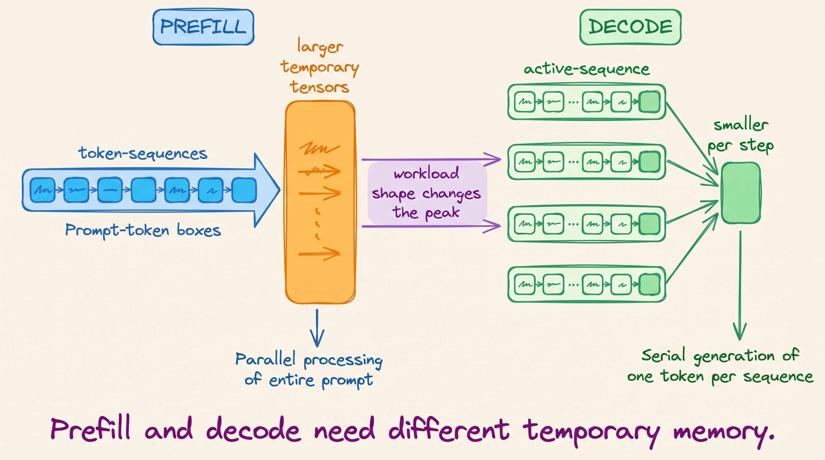
Different attention and matrix multiplication kernels request different workspace sizes. Memory-efficient kernels can lower the peak, while larger batches trade memory for better GPU utilization.
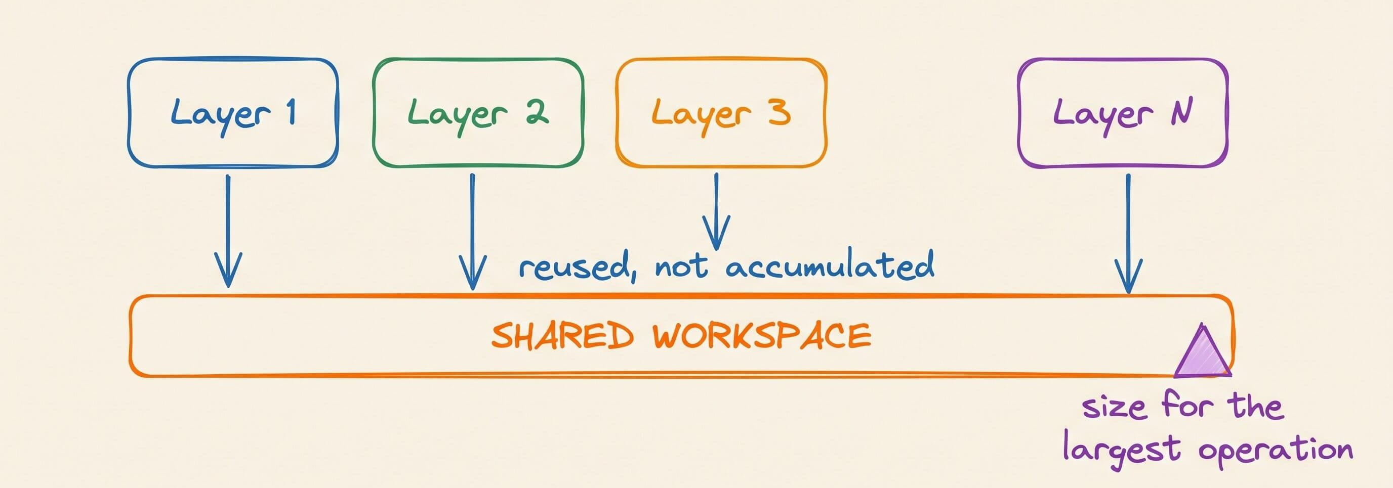
The GPU still needs enough free memory for this temporary peak. A workload can fail even when steady-state allocations appear to fit.
4. Runtime overhead
The final bucket contains CUDA contexts, loaded kernels, communication libraries, graph captures, scheduler buffers, allocator bookkeeping, and serving-framework state.
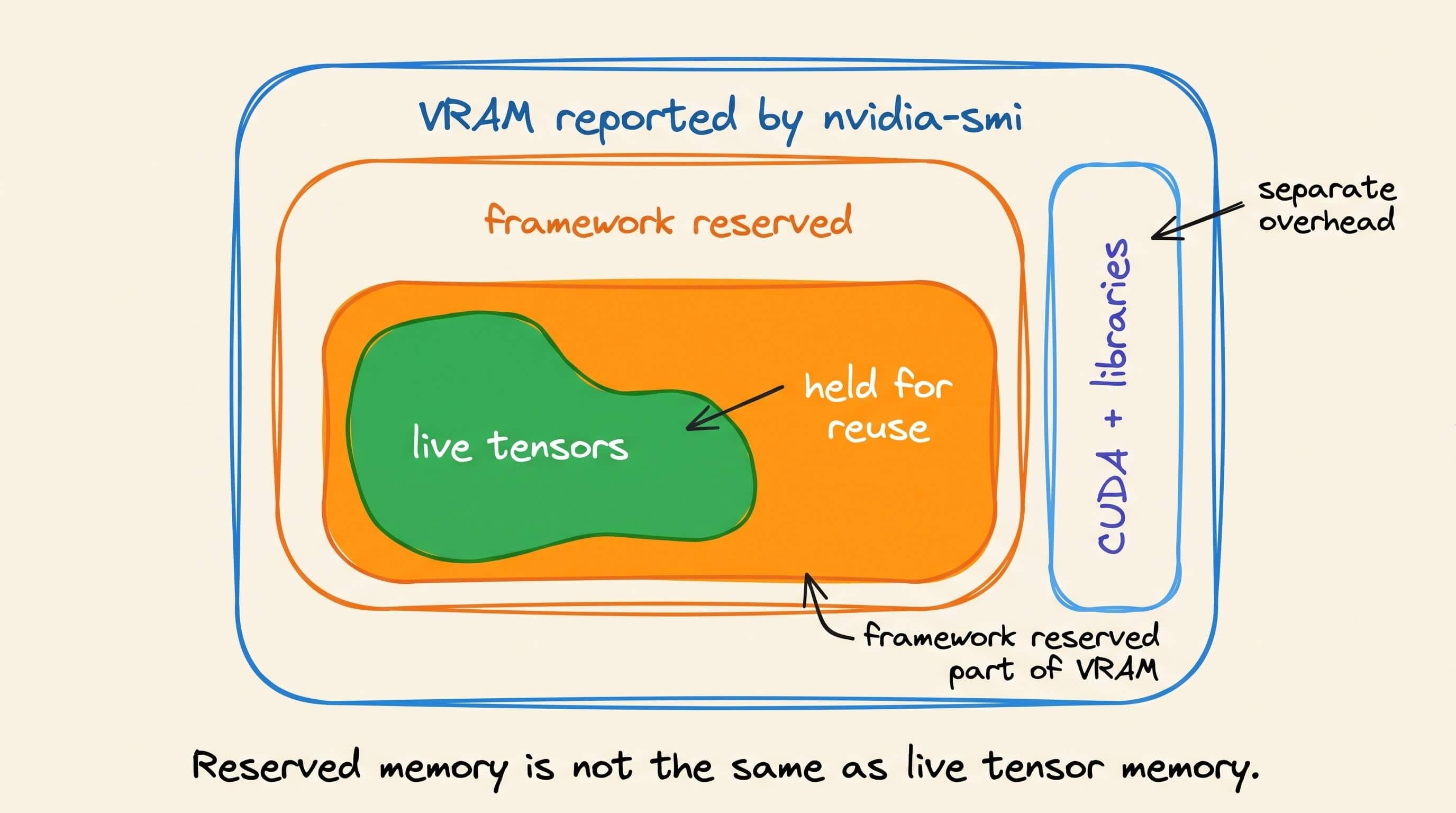
Caching allocators keep freed blocks reserved for reuse. Reserved memory can therefore exceed live tensor memory, while nvidia-smi can report more usage than the framework’s tensor counters.
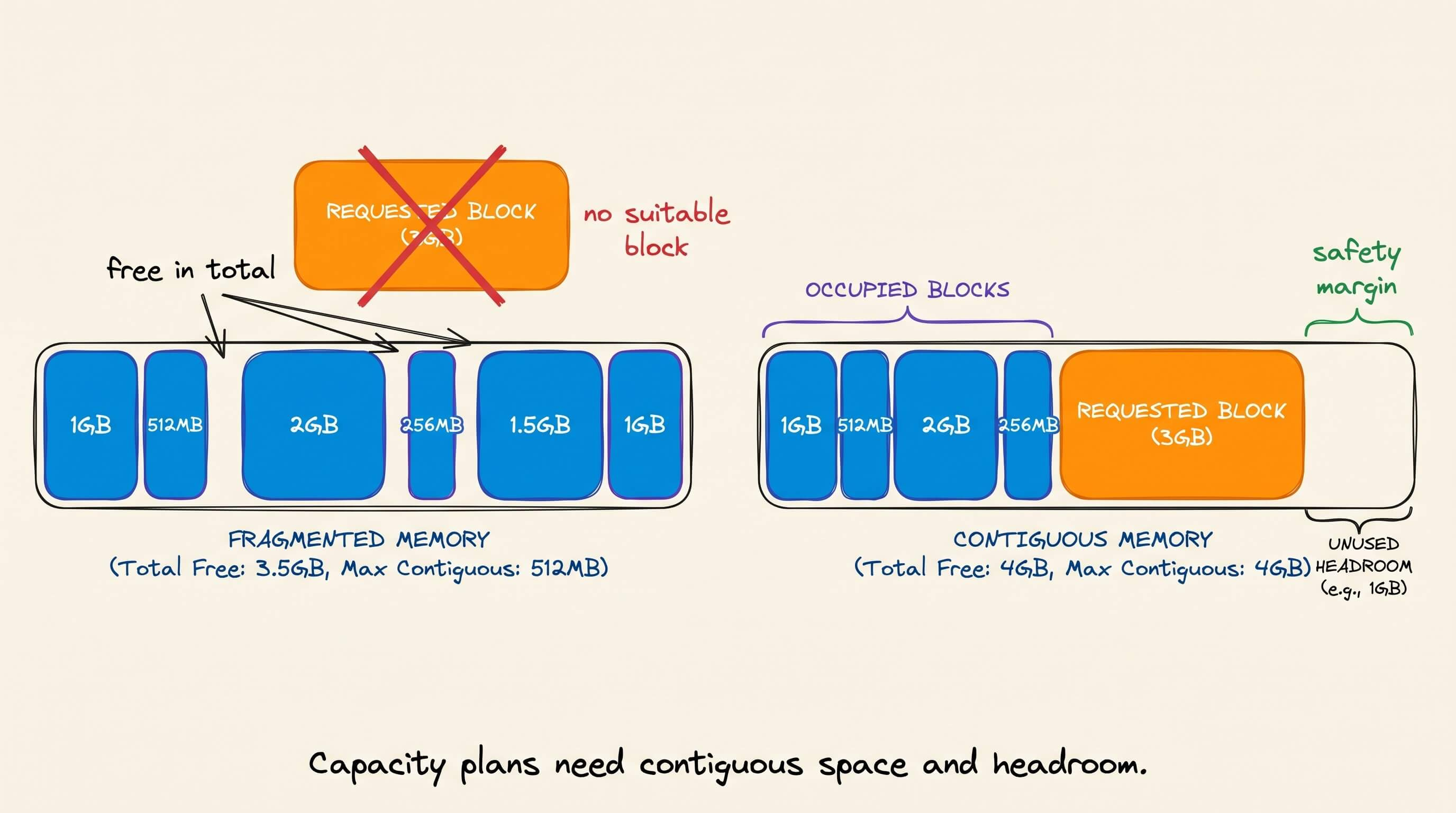
Fragmentation can leave enough free bytes in total but no suitable block for the next allocation. Capacity planning therefore needs headroom below the GPU’s physical limit.
The practical memory equation is:
Required VRAM ≈ weights + KV cache + peak activations and workspace + runtime overhead + safety margin
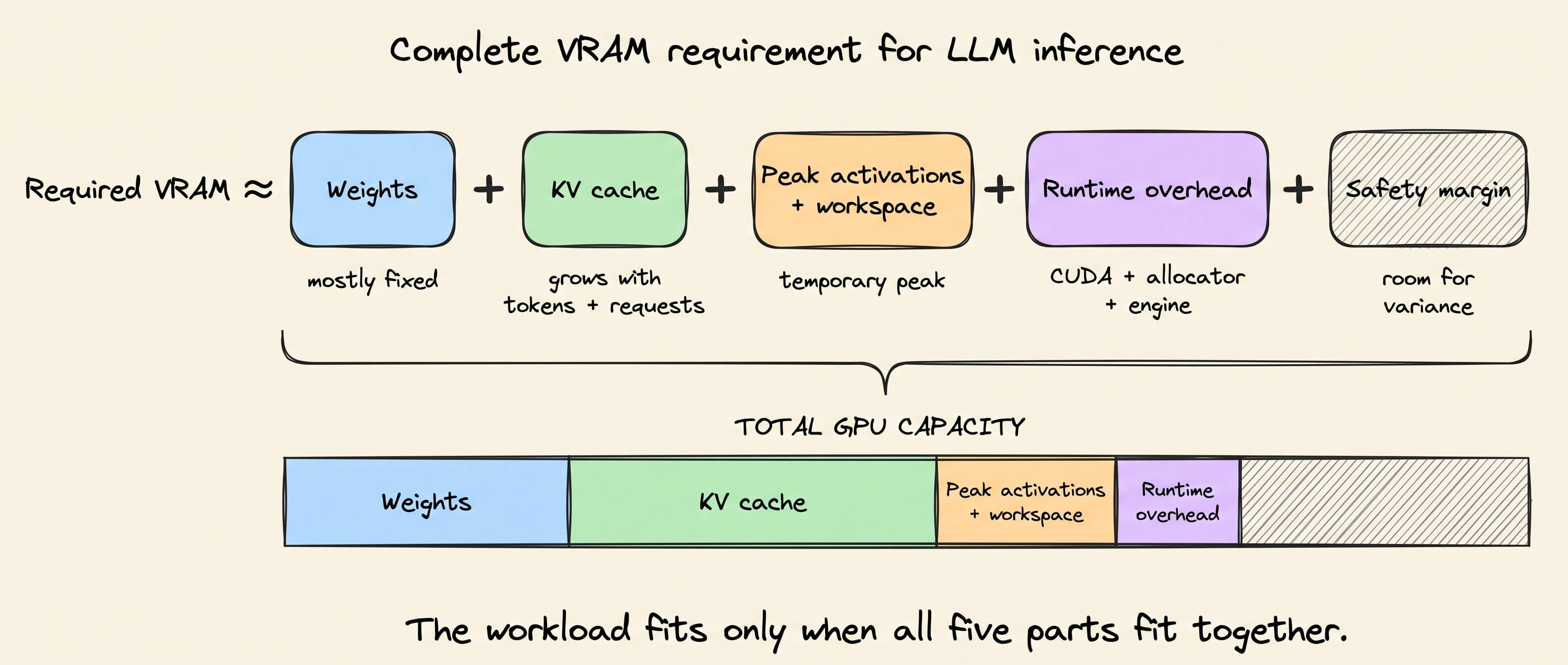
That equation explains why a model can load comfortably and still run out of memory after increasing the context window, concurrency, or batch size.
It also explains the wider performance problem. During decode, repeatedly reading weights and a growing KV cache can matter as much as raw compute capacity.
👉 Over to you: Which memory bucket has caused the most capacity problems in your inference workloads?
MCP meets agent skills
MCP already gave agents a standard way to connect to tools, resources, and external systems.
Now it also defines a standard way to discover and load Agent Skills directly from MCP servers.
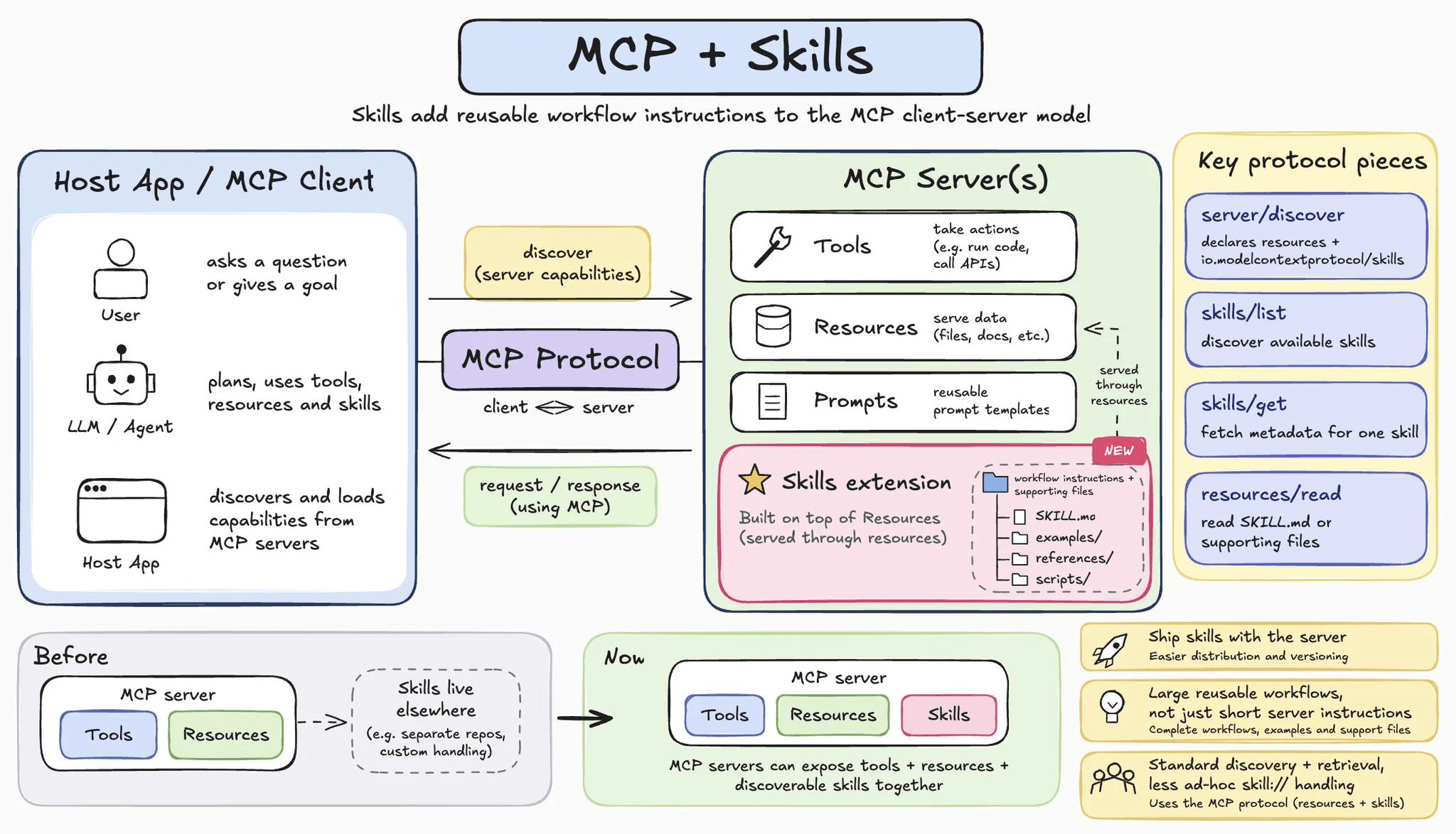
The flow is simple:
→ connect to MCP server
→ discover available skills
→ inspect skill metadata
→ load the relevant 𝗦𝗞𝗜𝗟𝗟.𝗺𝗱 only when needed
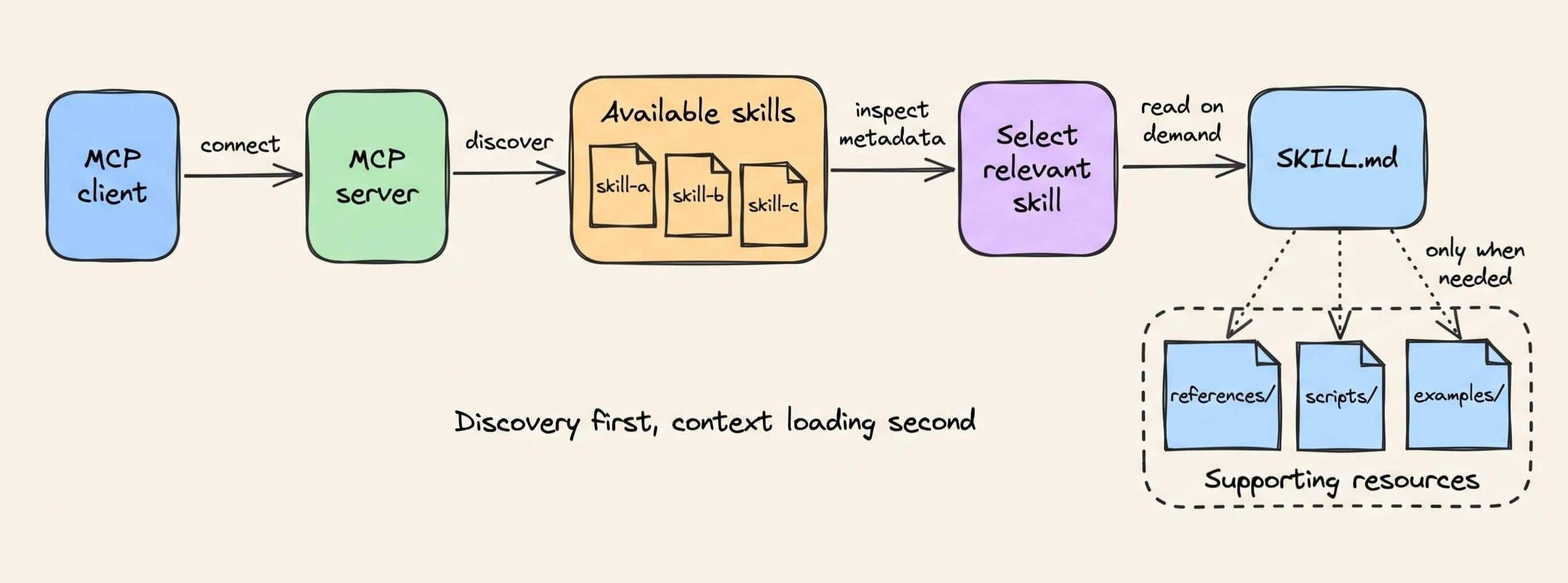
Under the hood, Skills are served through MCP’s existing Resources primitive.
That means 𝗦𝗞𝗜𝗟𝗟.𝗺𝗱, references, scripts, examples, and other supporting files are exposed as resources that the client can read on demand.
This is especially useful for context window management.
Instead of loading every workflow instruction upfront, the agent can first discover what skills are available and pull in only the one required for the current task.
A useful mental model is:
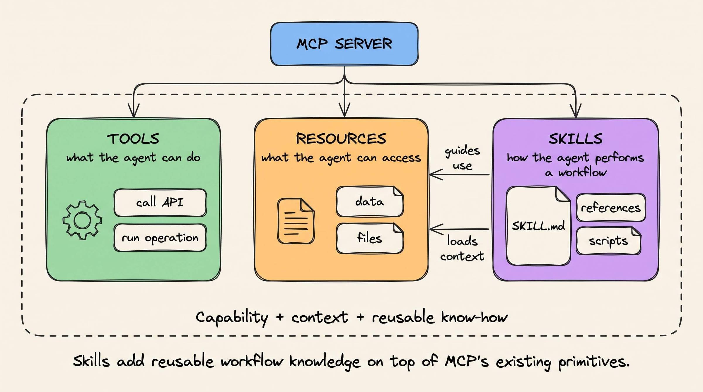
tools = what the agent can do
resources = what the agent can access
skills = how the agent should perform a reusable workflow
Previously, that workflow knowledge often lived separately in docs, repos, prompt files, or custom integrations.
Now the MCP server can expose the capability and the playbook for using it together.
So you get:
→ standardized skill discovery
→ on-demand context loading
→ cleaner distribution and versioning
→ reusable workflows that travel with the server
MCP was already the connection layer.
Skills now add a standardized way to ship reusable agent know-how on top of it.
The illustration below visually summarizes everything that we discussed so far.
Read more: https://github.com/modelcontextprotocol/ext-skills
Talking about MCPs, we covered everything you need to know about MCPs in the MCP crash course.
Part 1 covered MCP fundamentals, the architecture, context management, etc. →
Part 2 covered core capabilities, JSON-RPC communication, etc. →
Part 4 built a full-fledged MCP workflow using tools, resources, and prompts →
Part 5 taught how to integrate Sampling into MCP workflows →
Part 6 covered testing, security, and sandboxing in MCP Workflows →
Part 7 covered testing, security, and sandboxing in MCP Workflows →
Part 8 integrated MCPs with the most widely used agentic frameworks: LangGraph, LlamaIndex, CrewAI, and PydanticAI →
Part 9 covered using LangGraph MCP workflows to build a comprehensive real-world use case →
Good day!