

Turn any PDF, image, DOCX, and PPTX into clean MD
Datalab Marker v2 is an open-source parsing pipeline that runs up to 23.7 pages per second on a single B200 GPU.
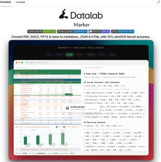
It outputs Markdown, JSON, or HTML, and under the hood it runs Surya 2, a single 650M parameter model that handles OCR, layout, reading order, and table recognition together, across more than 90 languages.
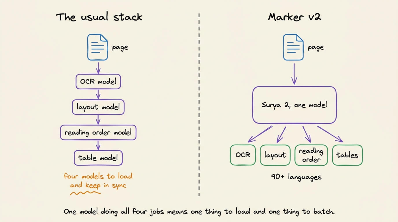
The usual way to scale parsing is to add more workers. Each worker loads its own copy of the model into GPU memory and feeds it one page at a time.
A GPU gets its speed from running many pages together in one pass, and a private copy fed one page at a time never gets that. It also sits idle while its worker reads the PDF and assembles the output on the CPU.
So you pay for multiple copies of the model and get close to the throughput of one.
Marker v2 runs many lightweight CPU workers that all talk to one shared Surya inference server, so pages from every worker batch together on one model instance that stays busy.
The parent process reads how much that server can handle and splits the capacity across the workers, so adding workers fills the pipeline instead of flooding it.
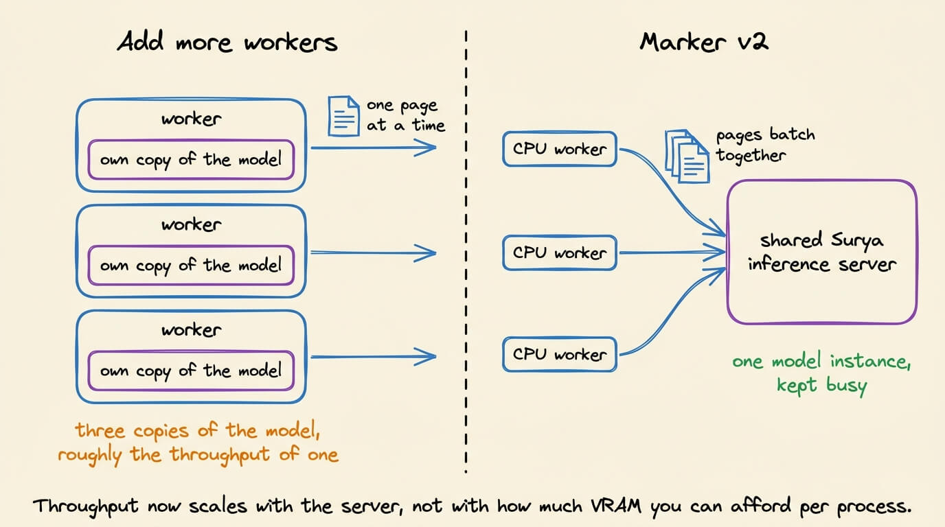
Throughput now scales with the server rather than with how much VRAM you can afford per process. That single B200 sustains 2.9 pages per second in balanced mode, 7.4 in fast, and 23.7 with OCR off.
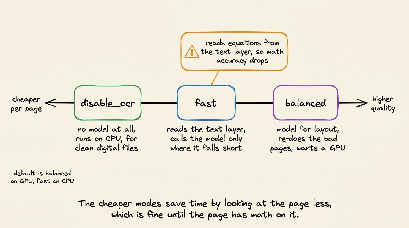
It also skips work it does not need. Marker reads the PDF’s own text layer first and calls the model only where that layer falls short, like scans, equations, and low-confidence tables.
Three modes let you set the trade-off:
balanced runs the model for layout and re-OCRs bad pages, highest quality, best on GPU
fast leans on the text layer with minimal model calls, far cheaper per page
disable_ocr skips the model entirely and runs on CPU for clean digital files
The default is balanced on GPU and fast on CPU or MPS.
One thing worth knowing before you switch. Fast mode reads equations out of the text layer instead of looking at the page, so math accuracy falls off sharply, and a math-heavy corpus should stay on balanced.
On olmOCR-bench, Allen AI’s harness of 1,403 PDFs, balanced scores 76.0% against MinerU at 72.7% while running over 5x more pages per second, and against Docling at 50.3%.
Why KV cache stores K and V vectors but never Q?
LLMs are autoregressive, so each token is predicted from every token before it, one at a time.
This autoregressive nature has a direct consequence inside the model.
A forward pass over <n> tokens produces <n> hidden states, but only the last one is projected to logits and is required to generate the next token.
So to understand why the KV cache just stores K and V vectors, we must backtrack to see how exactly the last hidden state is produced.
Let’s walk through this with a 10-token prompt.
1) Prefill:
All 10 tokens go through the model in one forward pass, in parallel (with causal masking), since the whole prompt is already known.
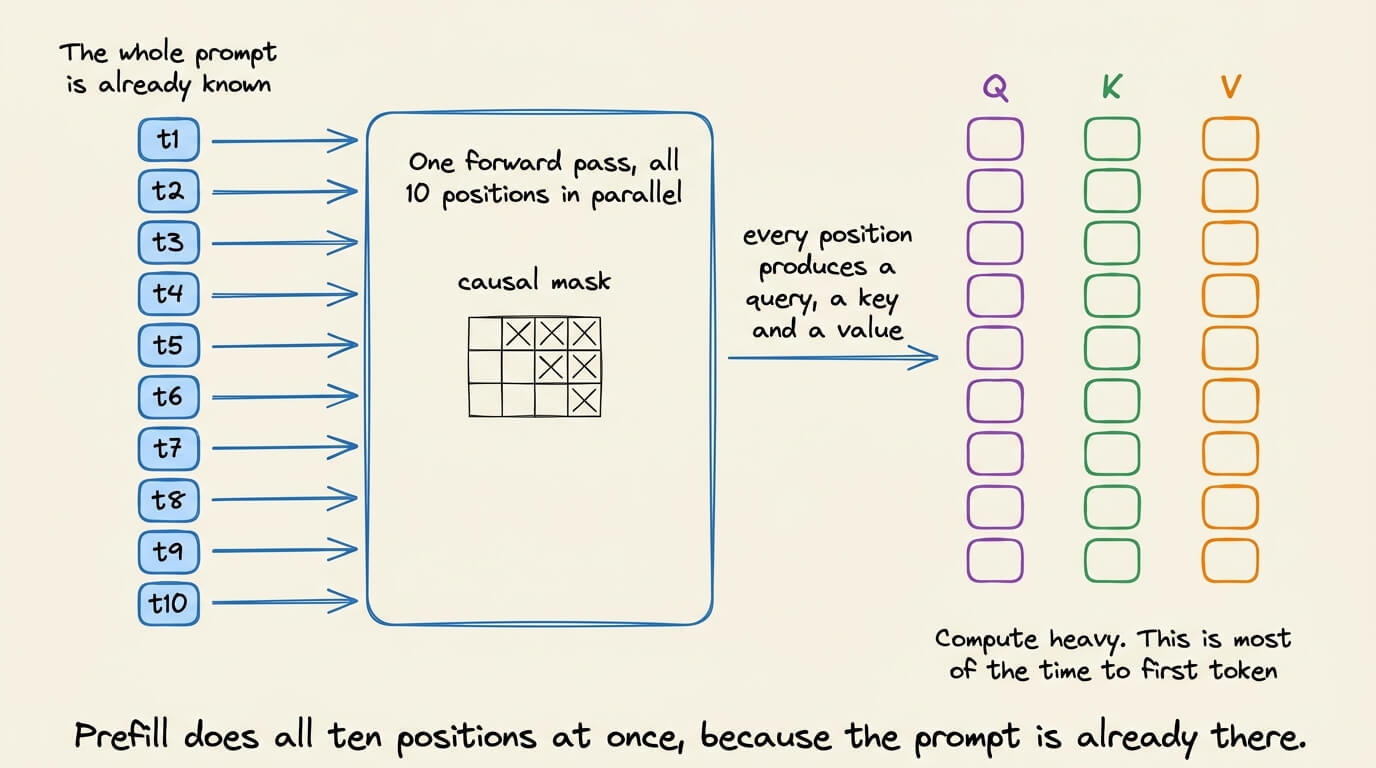
At every layer, each of the 10 positions produces a query, a key and a value vector, and attention at each position runs against all positions up to it.
This pass is compute-heavy, and it’s why the first token takes noticeably longer than the ones after it. TTFT is mostly prefill.
2) The first output token:
To generate the 11th token, only the 10th token’s hidden state is needed. So this is projected from the hidden-dim to vocab-dim to generate logits over vocab.
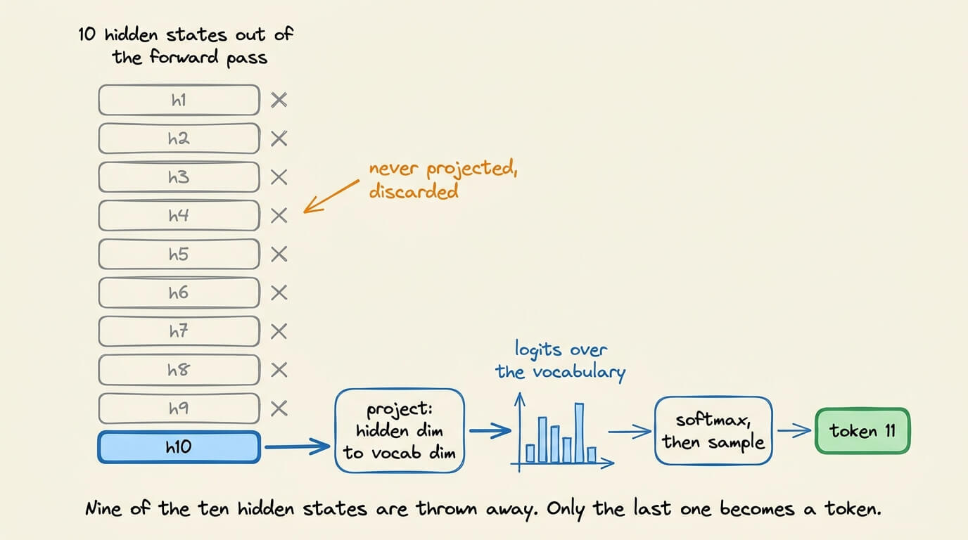
These logits then go through softmax and sampling to generate token 11.
3) Back-track the hidden state:
The last hidden state is the last row of the feedforward block’s output. The feedforward block is position-wise (it’s applied to each row independently), so that row comes from the last row of the attention output before it.
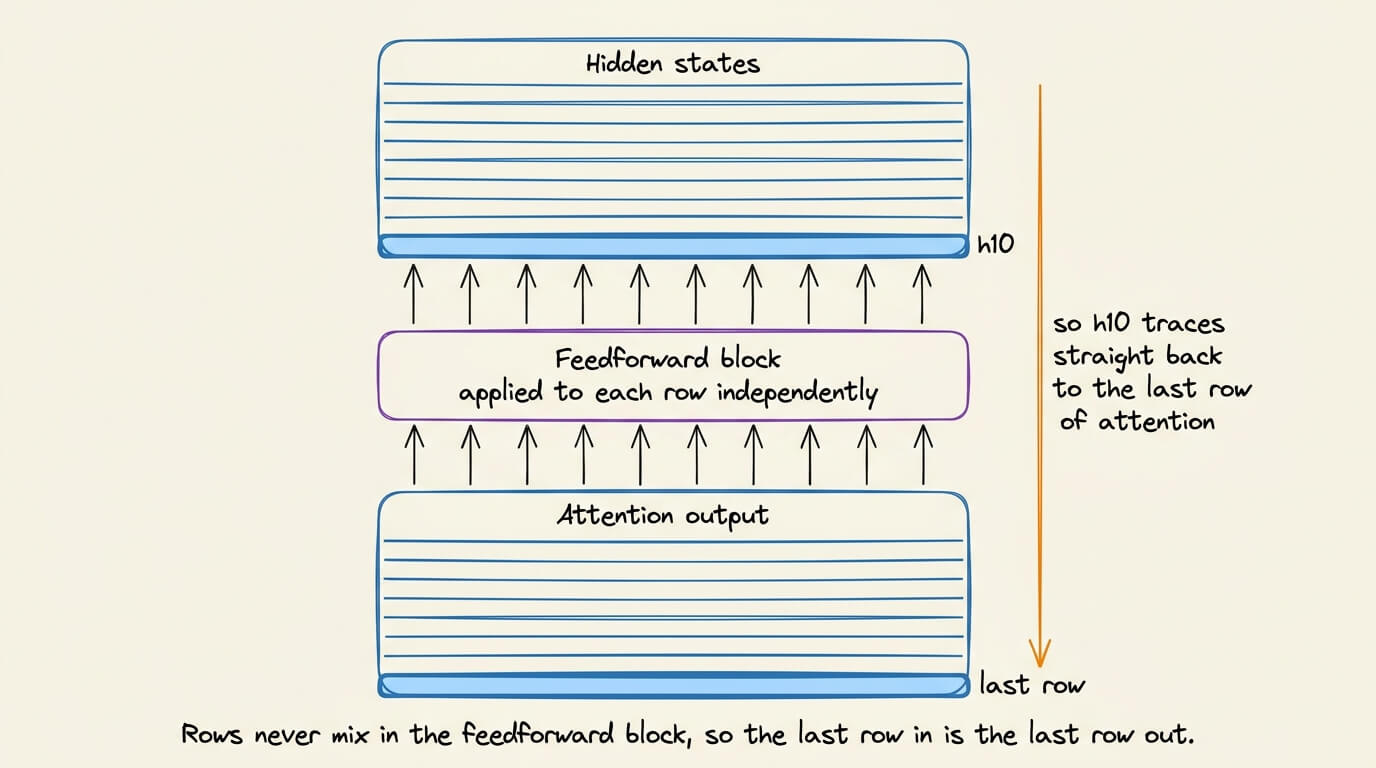
So now we need to see how the last row of attention is computed.
4) Attention matrix:
QKᵀ for a 10-token prompt will give a 10 × 10 matrix.
Row <i> will have the dot product of query <i> with every key.
Row 10 is therefore Q₁₀·K₁, Q₁₀·K₂, all the way to Q₁₀·K₁₀.
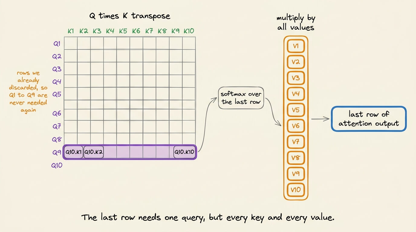
Notice that only Q₁₀ appears in it. Q₁ through Q₉ only belong to their corresponding rows 1-9, and those rows’ hidden states we already discarded because they were never needed.
The last row of attention goes through softmax and multiplies the full stack of value vectors, V₁ through V₁₀, to give the last row of the attention output.
So the last hidden state depends on exactly three things: Q₁₀, every key, and every value.
5) Generating token 12:
Token 11 is appended, and this time, we need row 11’s hidden state to generate token 12.
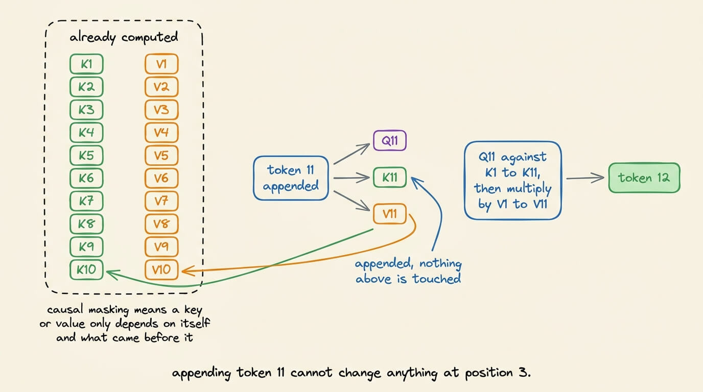
Mathematically, the attention operation turns out to be Q₁₁ against K₁ through K₁₁, then multiplied by V₁ through V₁₁.
K₁ through K₁₁ and V₁ through V₁₁ are bit-for-bit what prefill + first token produced since under causal masking, a token’s key and value depend on that token and the ones before it, never on anything after, so appending token 11 cannot change anything at position 3.
6) The cache state:
Overall, this implies that you just need to retain the keys and values at each decoding step, and compute only the new position’s Q, K, and V.
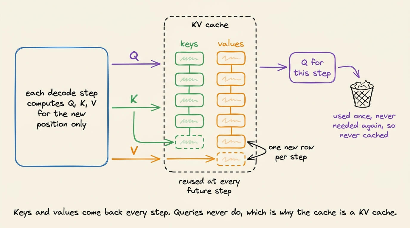
Each decode step requires one query vector, which is never used again, so they are never cached across the decoding process.
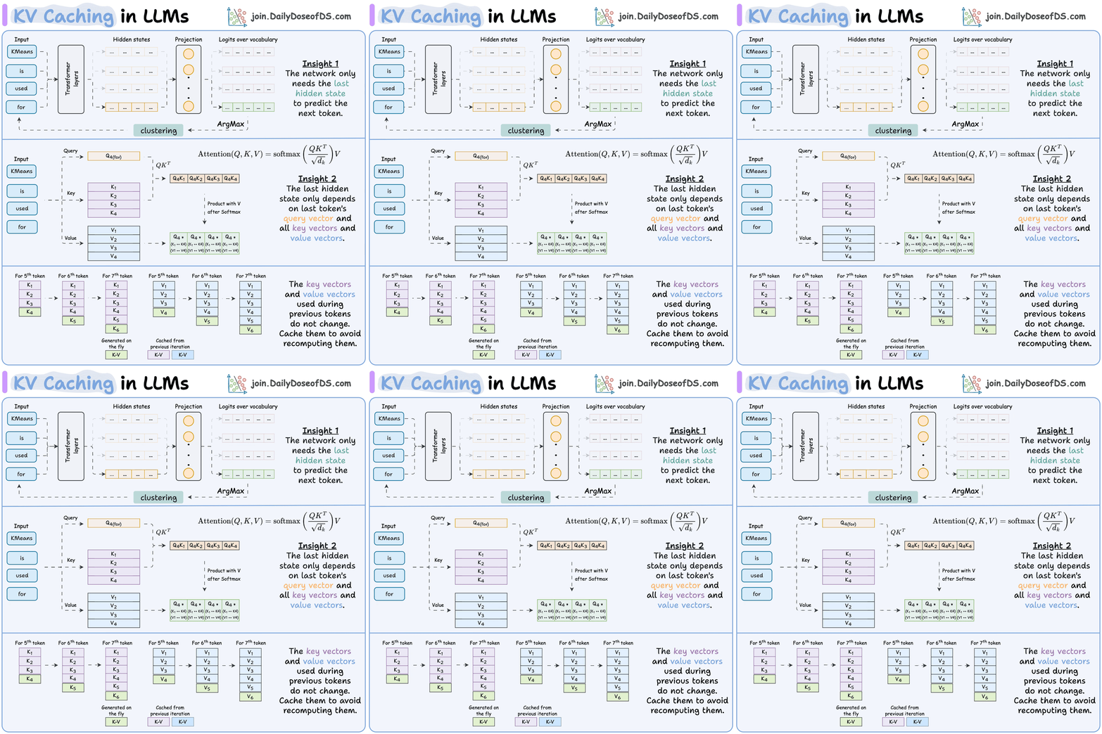
The visual below explains the entire process:
That said, KV cache is only one of four separate caching layers in an LLM stack.
The other three are prefix caching on the server, prompt caching billed by a provider, and a semantic cache that skips the model entirely.
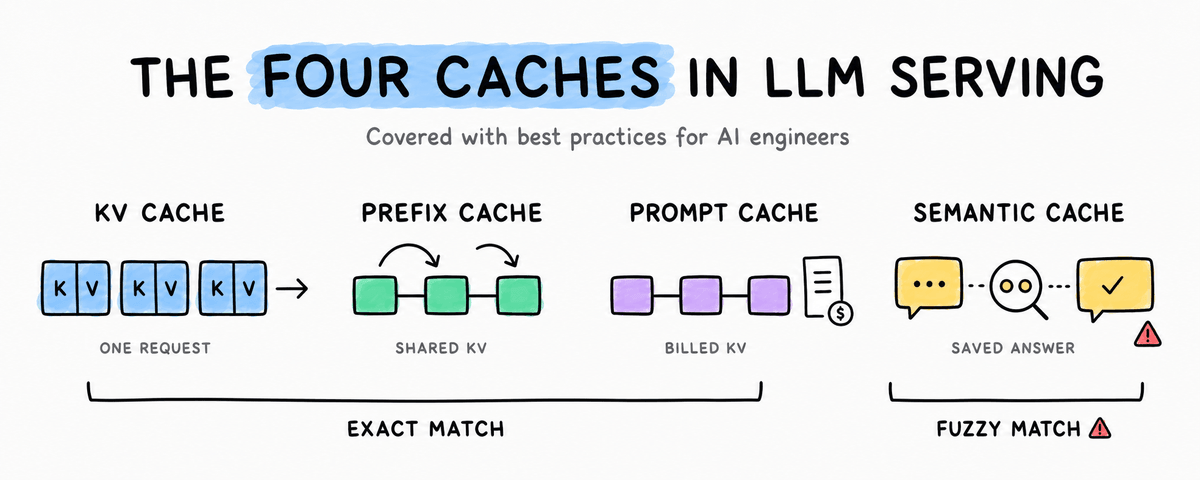
We wrote a full breakdown of all four caches in LLM serving that you should know as an AI engineer, with code for each.
Good day!
P.S. For those wanting to develop “Industry ML” expertise:

At the end of the day, all businesses care about impact. That’s it!
Can you reduce costs?
Drive revenue?
Can you scale ML models?
Predict trends before they happen?
We have discussed several other topics (with implementations) that align with such topics.
Here are some of them:
Learn everything about MCPs in this crash course with 9 parts →
Learn how to build Agentic systems in a crash course with 14 parts.
Learn how to build real-world RAG apps and evaluate and scale them in this crash course.
Learn sophisticated graph architectures and how to train them on graph data.
So many real-world NLP systems rely on pairwise context scoring. Learn scalable approaches here.
Learn how to run large models on small devices using Quantization techniques.
Learn how to generate prediction intervals or sets with strong statistical guarantees for increasing trust using Conformal Predictions.
Learn how to identify causal relationships and answer business questions using causal inference in this crash course.
Learn how to scale and implement ML model training in this practical guide.
Learn techniques to reliably test new models in production.
Learn how to build privacy-first ML systems using Federated Learning.
Learn 6 techniques with implementation to compress ML models.
All these resources will help you cultivate key skills that businesses and companies care about the most.