

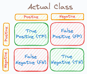
When we build any binary classification model, it is natural to create a confusion matrix:
But have you ever struggled to quickly and intuitively classify a prediction as one of TP, TN, FP, and FN?

If yes, then today, let me share one of the simplest techniques I always use.
If you love to watch, check out the video above.
If you love to read, continue reading below.
Let’s dive in!
When labeling any binary classification prediction, you just need to ask these two questions:
Question 1) Did the model get it right?
Quite intuitively, the answer will be one of the following:
Yes (or True)
No (or False).
Question 2) What was the predicted class?
The answer will be:
Positive, or
Negative
Next, just combine the above two answers to get the final label.
And you’re done!
For instance, say the actual and predicted class were positive.

Question 1) Did the model get it right?
Of course, it did.
So the answer is yes (or TRUE).
Question 2) What was the predicted class?
The answer is POSITIVE.
The final label: TRUE POSITIVE.
Simple, right?
The following visual neatly summarizes this:

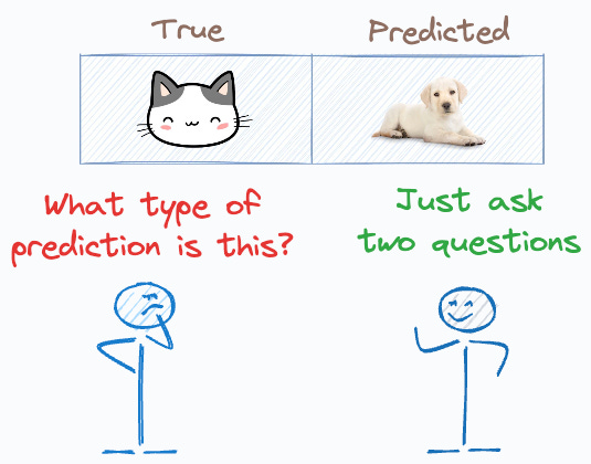
As an exercise, try to complete the table below.
Consider:
The cat class → Positive.
The dog class → Negative.

Let me know your answer in the comments.
👉 Over to you: Do you know any other special techniques to label binary classification predictions? Let me know :)
Thanks for reading!
Extended piece #1
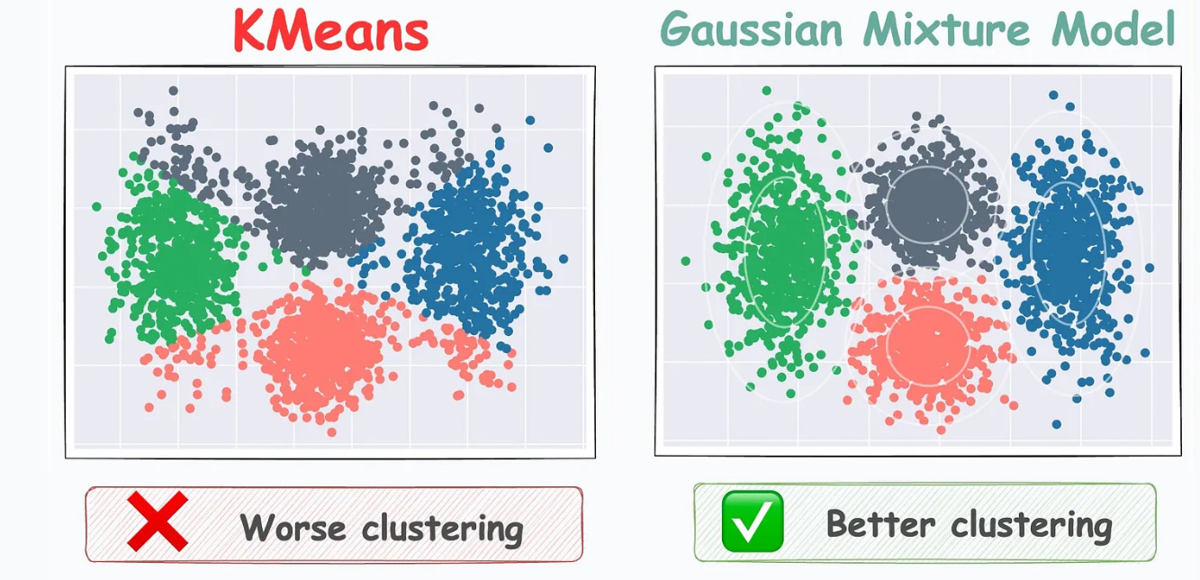
KMeans has limited applicability to real-world datasets.
For instance:
It can only produce globular clusters.
It performs a hard assignment. There are no probabilistic estimates of each data point belonging to each cluster.
It does not take into account cluster variance, etc.
Gaussian Mixture Models are often a superior algorithm in this respect.
They can be thought of as a more flexible twin of KMeans.
In 2 dimensions:

KMeans can only create circular clusters
GMM can create oval-shaped clusters.
The effectiveness of GMMs over KMeans is evident from the image below.
To get into more details, I covered them in-depth here: Gaussian Mixture Models.
Extended piece #2
Linear regression is powerful, but it makes some strict assumptions about the type of data it can model, as depicted below.

Can you be sure that these assumptions will never break?
Nothing stops real-world datasets from violating these assumptions.
That is why being aware of linear regression’s extensions is immensely important.
Generalized linear models (GLMs) precisely do that.
They relax the assumptions of linear regression to make linear models more adaptable to real-world datasets.
👉 Read it here: Generalized linear models (GLMs).
Note: I hired Mustafa Marzouk to create today’s video. You can find him on LinkedIn here. He creates awesome animations in Manim.
Are you preparing for ML/DS interviews or want to upskill at your current job?
Every week, I publish in-depth ML dives. The topics align with the practical skills that typical ML/DS roles demand.
Join below to unlock all full articles:
👉 If you love reading this newsletter, share it with friends!
👉 Tell the world what makes this newsletter special for you by leaving a review here :)
